Timeline

Hess discovers cosmic rays

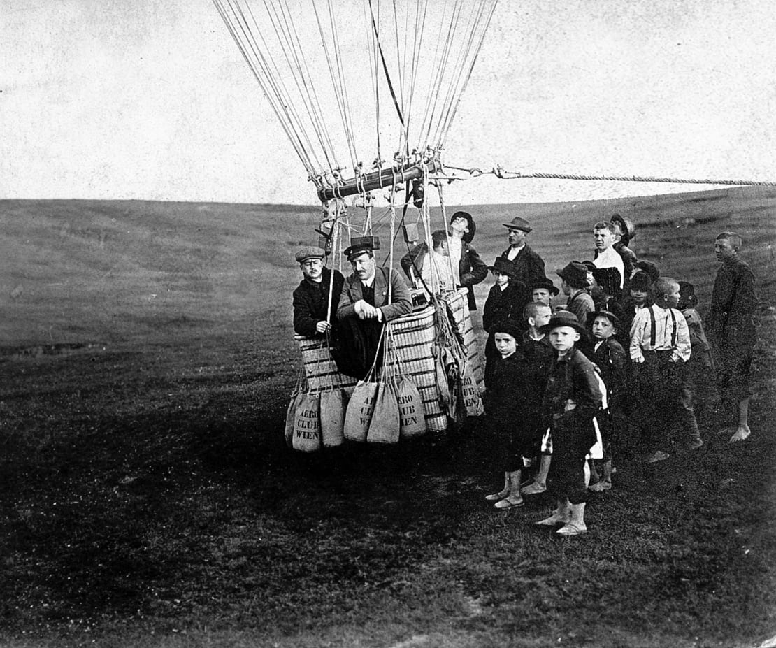
In 1911 and 1912, Austrian physicist Victor Franz Hess carried out a series of experiments measuring radiation in Earth’s atmosphere by ascending in a hydrogen balloon with ionization measuring devices. At the time, the prevailing theory was that radiation was coming from rocks on Earth; if this was the case, the ionization rate should be lower at higher altitudes. During earlier experiments and Hess’s previous flights, the ionization rate did not change, leading them to believe that the radiation couldn’t be coming from Earth.

On August 7, 1912, Hess took a balloon flight 5,300 meters (17,400 feet) above Germany. That day, there was a near-total eclipse of the sun, but the ionization rate was no lower, showing that the radiation couldn’t be coming from the sun. In fact, it was coming from much farther away in outer space. Hess had discovered cosmic rays.

Hess received the 1936 Nobel Prize in Physics for this discovery.

Pauli postulates hypothetical “neutron” particle

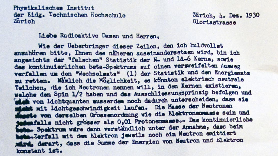
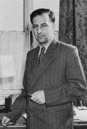
Before 1930, there was a baffling issue in nuclear physics: a certain nuclear decay called beta decay appeared to lose energy, which contradicted the law of the conservation of energy. So Wolfgang Pauli, age 30, had the idea that maybe there was a lightweight particle produced in the decay that was responsible for the missing energy. At the time, Pauli dubbed the particle a “neutron,” but the particle he hypothesized would eventually be named the neutrino.

On December 4, 1930, Pauli wrote a letter to a group of nuclear physicists outlining his idea for what is now known as the neutrino. It opened, “Dear radioactive ladies and gentlemen…” Read more about the letter here.

Fermi develops his theory of weak interaction that includes the neutrino

Italian physicist Enrico Fermi introduced the name “neutrino” in 1932 at a conference in Paris. Meaning “little neutral one” in Italian, “neutrino” was adopted to differentiate Pauli’s hypothesized “neutron” particle from a massive nuclear particle discovered by James Chadwick in 1932, which was also called the neutron.

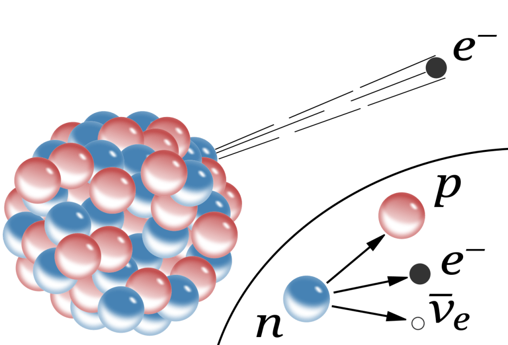
In 1933, Fermi developed his theory of beta decay that included the neutrino, which he assumed to be massless (or otherwise have a very small mass) and chargeless. Fermi’s theory was the precursor to the theory of the weak nuclear force—the third fundamental force of nature (after gravity and electromagnetism but before the strong nuclear force). The theory also showed that beta decay could run in reverse, which happens to be the underlying principle that allows IceCube to work.

Cowan and Reines et al. discover the neutrino experimentally

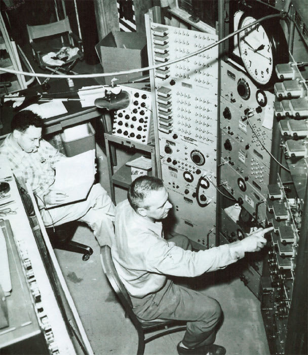
During the 1950s, physicists Clyde L. Cowan and Frederick Reines conducted a series of experiments to detect the neutrino. They planned to do this using inverse beta decay (one of the interactions also seen by IceCube), in which a neutrino (more specifically an electron antineutrino) interacts with a proton inside an atomic nucleus producing  a neutron and a positron.

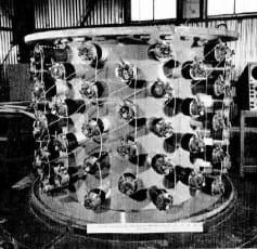
The idea was to detect neutrinos by looking for the particles it left behind after it interacted with something. They set up an experiment using a tank of water and layers of liquid scintillators that could pick up signals from the secondary particles; a nuclear reactor provided the neutrinos. When a neutrino interacted with a proton in the water tank, the resulting particles would leave signature tracks in the liquid scintillator, revealing the neutrino’s presence.

They first performed the experiment at the Hanford Site in Washington, but the cosmic-ray background muddied their data too much. So they moved to the Savannah River Plant in South Carolina where they had better shielding against cosmic rays—and that’s where they got their definitive results. They were able to identify about three neutrinos per hour in the many months of data they had collected.

The results, which were consistent with the predictions in Fermi’s theory of beta decay, were published in Science in July 1956. Reines was awarded a Nobel Prize in Physics for this experiment in 1995; Cowan died in 1974 and was thus ineligible.

Read more about it here, here, here, and here.

Pontecorvo predicts neutrino flavor oscillations

Today, the idea of neutrino oscillations is indispensable to the field of neutrino physics. But in 1957, when it was first suggested by Italian physicist Bruno Pontecorvo, it was a wild notion. He thought that there was an analogy between leptons and hadrons and that neutrinos could oscillate in an analogous way to neutral kaon mixing. But, in order to oscillate, neutrinos must have mass; whether they did was unknown at the time. In addition, oscillation today means to change from one type of neutrino to another, but in 1957, there was only one known type, now called “flavor,” of neutrino.

Neutrino oscillations would be first observed experimentally 40 years later, after Pontecorvo’s death. But his idea of neutrino masses, mixing, and oscillations established a new field of neutrino research and changed neutrino physics forever. Read more here.

Markov proposes installing neutrino detectors underwater

At the 1960 Rochester Conference, Soviet physicist Moisey M. Markov proposed an idea “…to install detectors deep in a lake or a sea and to determine the direction of charged particles with the help of Cherenkov radiation.” This concept led to the series of underwater and in-ice telescopes that would eventually result in the IceCube Neutrino Observatory.

Linsley detects first 10²⁰ eV cosmic ray

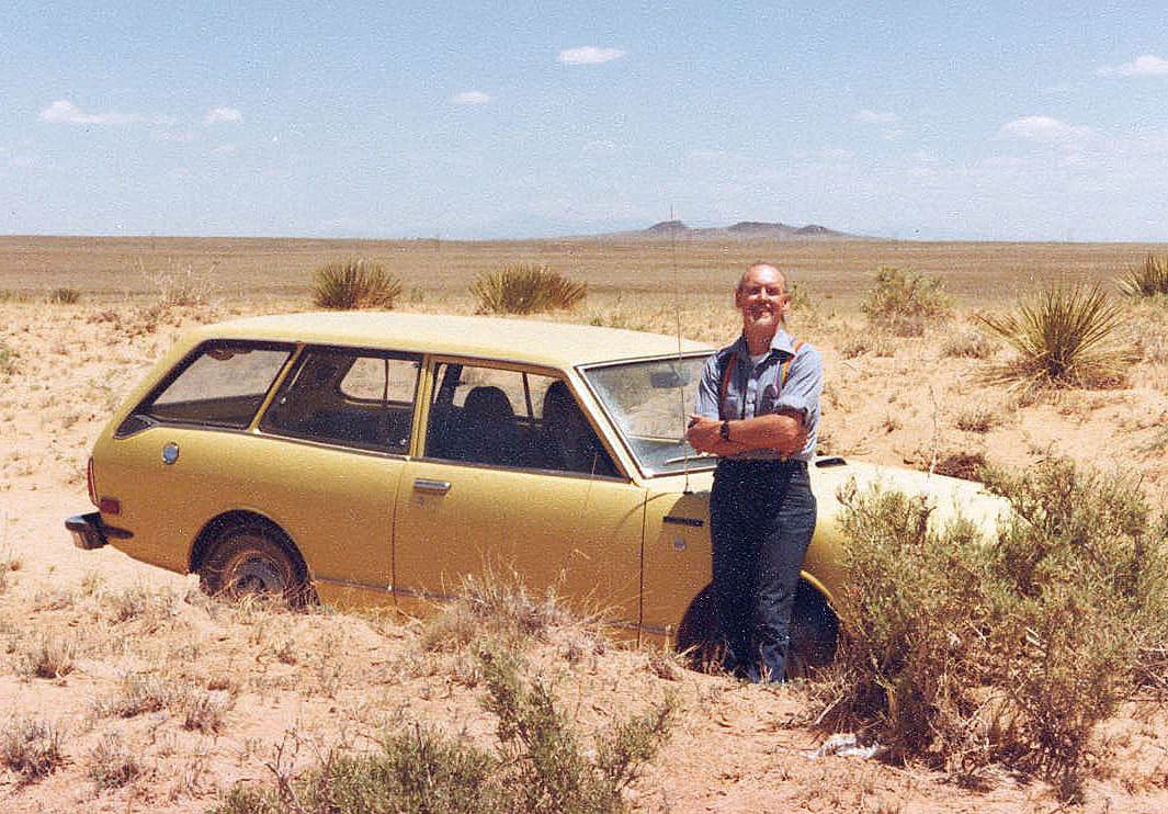
In the late 1950s, American physicist John Linsley worked with Livio Scarsi from the University of Milan to build an array of nineteen plastic scintillation detectors at Volcano Ranch near Albuquerque, New Mexico. On February 22, 1962, using these ground-based detectors, Linsley identified the first cosmic ray with an energy higher than 10²⁰ eV—the highest energy cosmic ray particle ever detected at the time. Their observations suggested that not all cosmic rays are confined to the galaxy, clarified the structure of air showers, and provided the first evidence of ultra-high-energy cosmic ray composition and arrival directions.

Lederman, Steinberger, and Schwartz et al. report the discovery of a second neutrino flavor

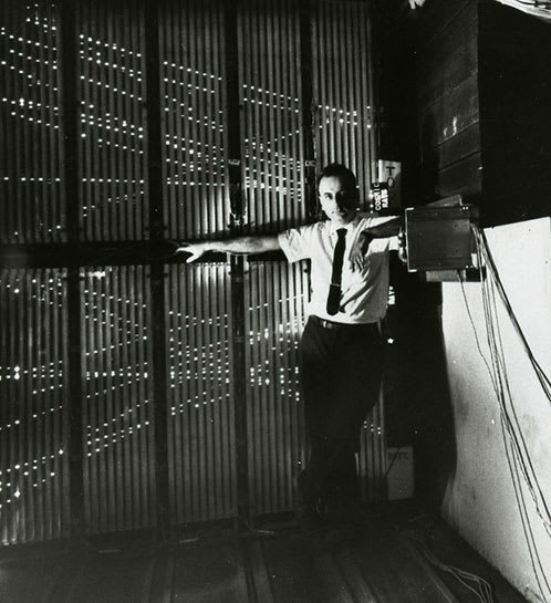
American physicists Leon Lederman, Melvin Schwartz, and Jack Steinberger joined forces to search for another type of neutrino at Brookhaven National Laboratory on Long Island, New York. At the time, only the electron neutrino was known.

Their experiment shot a powerful beam of protons at a beryllium target, producing large numbers of pions that would then decay into muons and neutrinos. Only the latter particles could pass through the wall into a neon-filled detector called a spark chamber. There, neutrinos that interacted with protons in the aluminum plates produced muons that could be detected and photographed by their spark trails—proving the existence of muon-neutrinos.

They reported their results in a 1966 paper. All three physicists received the 1988 Nobel Prize in Physics for their discovery. Read more here.

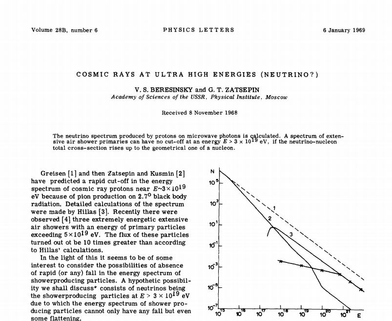
Berezinsky, Zatsepin, Greisen, and Kuzmin propose cosmogenic neutrino production theory

In 1969, Veniamin S. Berezinsky and Georgy T. Zatsepin suggested that it was possible to observe ultra-high-energy neutrinos known as cosmogenic neutrinos. By that time, Zatsepin, American physicist Kenneth I. Greisen, and Russian theorist and cosmologist Vadim A. Kuzmin had independently discovered an upper limit of cosmic ray energies. They realized that ultra-high-energy cosmic rays should interact with photons in the cosmic microwave background to produce neutrinos at ultrahigh energies. These cosmogenic neutrinos were estimated to have energies between a PeV (10¹⁵ eV) and a million PeV (10²¹ eV). Today, they are called GZK neutrinos for Greisen, Zatsepin, and Kuzmin.

The GZK mechanism produces a “guaranteed” flux of extremely high energy neutrinos. However, the neutrino flux depends on the composition of the cosmic rays that produce it. If the extremely high energy cosmic rays are primarily protons, the GZK neutrino should be observable with the next generation of neutrino telescopes and radio experiments. If extremely high energy cosmic rays are composed of heavier nuclei, the neutrino flux will be much lower and difficult to observe.

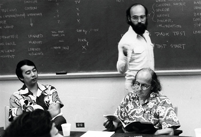
First of a series of DUMAND workshops advances the concept of neutrino telescopes

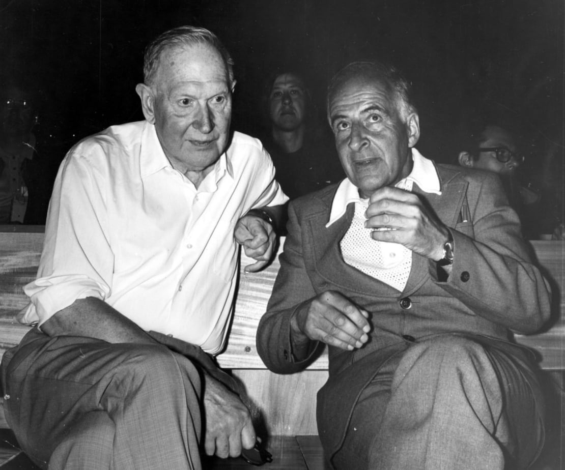
At the 1973 International Cosmic Ray Conference, a group of physicists including Frederick Reines, John Learned, Georgy Zatsepin, and Saburo Miyake founded a committee to explore the feasibility of DUMAND (Deep Underwater Muon and Neutrino Detector), a Markov-type instrument.

In 1975, they held the first of a now-legendary series of DUMAND workshops that took place regularly over the next decade. Co-led by Learned and Reines, the committee decided the detector was to be placed at a 4,800-meter depth in the Pacific Ocean off the Big Island of Hawaii. It was funded in 1980. However, the short-circuiting of a deployed test string and other circumstances led the US Department of Energy to terminate its support for DUMAND in 1995. Despite its failure as a neutrino detector, the undertaking pioneered many of the techniques used today in IceCube and other neutrino telescopes.

Read more here and here.

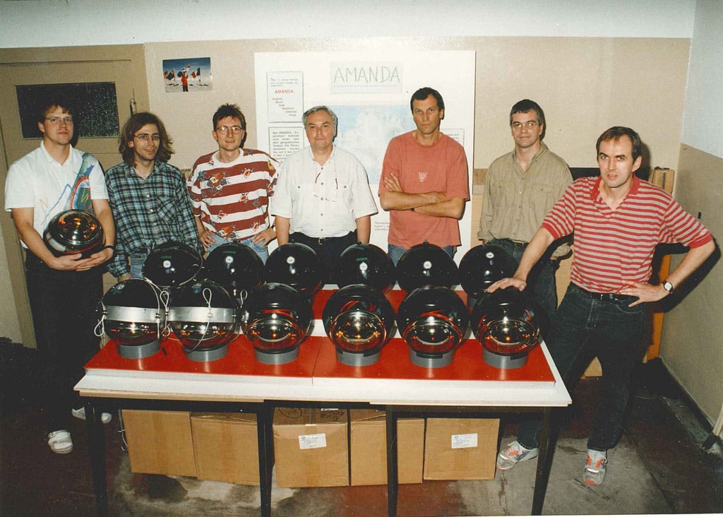
AMANDA test string proves feasibility of an in-ice neutrino detector

In a 1991 Nature paper, Francis Halzen, Bob Morse, Buford Price, and other collaborators described the initial results of the AMANDA (Antarctic Muon And Neutrino Detector Array) project, which tested the feasibility of using ice to detect neutrinos with instruments deployed on the summit of the Greenland ice sheet. The paper outlined the reasons why deploying a larger detector in the Antarctic ice sheet would be a good idea. Today, the paper’s abstract has proven to be incredibly prescient:

“Detection of the small flux of extraterrestrial neutrinos expected at energies above 1 TeV, and identification of their astrophysical point sources, will require neutrino telescopes with effective areas measured in square kilometres—much larger than detectors now existing. Such a device can be built only by using some naturally occurring detecting medium of enormous extent: deep Antarctic ice is a strong candidate. A neutrino telescope could be constructed by drilling holes in the ice with hot water into which photomultiplier tubes could be placed to a depth of 1 km. Neutrinos would be recorded, as in underground neutrino detectors using water as the medium, by the observation of Cerenkov radiation from secondary muons. … Our results suggest that a full-scale Antarctic ice detector is technically quite feasible.”

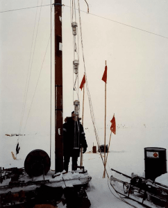
AMANDA construction at the South Pole begins

The first phase of the AMANDA array, called AMANDA-A, was installed during the 1993-1994 austral summer. Holes were drilled using a hot-water drilling technique that had been developed by glaciologists. AMANDA-A consisted of four strings with 20 optical modules each, spaced 10 meters apart. The strings were deployed between depths of 800 and 1,000 meters. As it turned out, ice at 1,000-meter depths was too shallow for their purposes—there were too many air bubbles, which would prohibit the detector from seeing accurate signals from neutrino interactions.

In later construction campaigns (AMANDA-B4 in 1995-1996, AMANDA-B10 in 1996-1997, and AMANDA-II in 1998-2000), the AMANDA team deployed strings at depths of 1,500 meters and deeper in search of more transparent ice. The AMANDA Collaboration would conclude that ice is transparent below approximately 1,500 meters—information that was later used in the design of the IceCube Neutrino Observatory.

Lake Baikal neutrino telescope detects neutrinos

Another Markov-style neutrino detector was built in Lake Baikal, Russia. The largest and deepest freshwater lake in the world, Lake Baikal had extremely clear and unpolluted water whose surface froze in the winter, making it an ideal environment in which to deploy a neutrino telescope.

Just after its four strings of sensors were installed, in April and May 1996, the Baikal telescope detected the first-ever “upgoing” neutrino candidates in an underwater detector—two of them! They had come through Earth and up through the detector. However, they were created by cosmic ray interactions in Earth’s atmosphere, not in extreme astrophysical environments or events.

IceCube submits proposal for cubic-kilometer South Pole neutrino detector

In November 1999, the fledgling IceCube Collaboration (mostly members of the AMANDA Collaboration) submitted a 67-page proposal for a cubic-kilometer neutrino detector at the South Pole to the US National Science Foundation and to partners in Belgium, Germany, and Sweden. In it, the University of Wisconsin–Madison was designated the lead institution, Francis Halzen was principal investigator, and Bob Paulos was project manager.

AMANDA-II neutrino detector at the South Pole is completed

AMANDA’s later development stage was known as AMANDA-II. Nine additional strings were added in 2000, bringing the array to a total of 677 optical modules mounted on 19 separate strings that were spread out in a rough circle with a diameter of 200 meters. AMANDA-II operated through 2009.

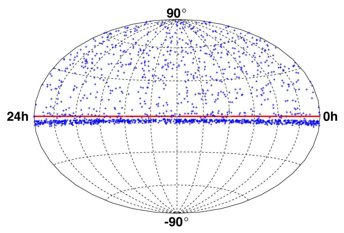
AMANDA publishes first neutrino sky map in Nature

On March 22, 2001, the initial results from AMANDA came out in Nature. Over 138 days in 1997, AMANDA’s sensors saw 263 high-energy neutrinos, and they produced a map showing the origins of those particles in the sky. As Francis Halzen told a Nature writer, “This is a proof of concept showing that we can build a neutrino telescope in ice.”

This paper helped pave the way for the future IceCube Neutrino Observatory; the final line in its abstract says, “These results establish a technology with which to build a kilometre-scale neutrino observatory necessary for astrophysical observations.”

National Science Board approves initial funding for IceCube construction

In March 2002, the National Science Board (NSB), the 24-member policy body for the National Science Foundation (NSF), approved a $15 million award for the IceCube project. A year later in May 2003, the NSB would approve up to $24.54 million for the University of Wisconsin and U.S. Antarctic Program logistics and support contractors to complete the first phase of the IceCube Neutrino Observatory at the South Pole. NSF would eventually contribute $242 million toward the total project cost of $279 million.

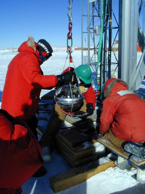
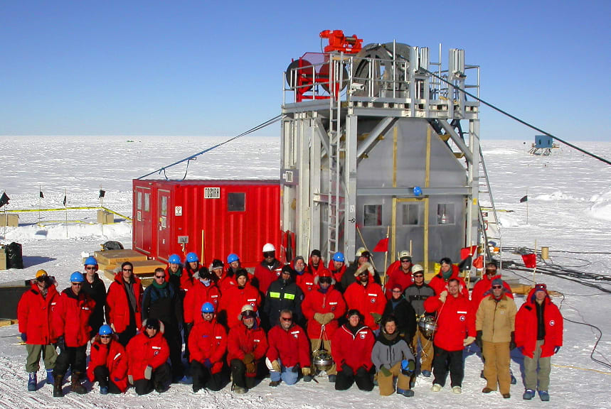
IceCube construction begins at the South Pole

How do you construct a cubic kilometer detector in the Antarctic ice? Slowly, carefully…and with a 4.8-megawatt hot-water drill that can penetrate more than two kilometers into the ice in less than two days.

After the hot-water drill bores cleanly through the ice sheet, deployment specialists attach optical sensors to cable strings (each string gets 60 sensors) and lower them to depths between 1,450 and 2,450 meters. The ice itself at these depths is completely dark and optically ultratransparent (no bubbles here!). Deployment takes about 11 hours per string. One string was deployed in the Antarctic summer of 2004: #21 in the numbering scheme of the array.

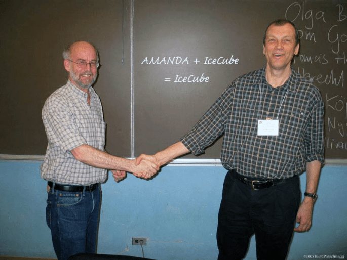
AMANDA and IceCube merge to form a single IceCube Collaboration

On March 20, 2005, after nine years of operation, AMANDA officially became part of IceCube!

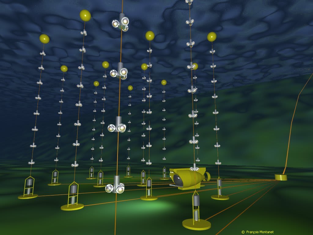
ANTARES neutrino detector in the Mediterranean Sea is completed

In the same vein as DUMAND, the ANTARES (Astronomy with a Neutrino Telescope and Abyss environmental RESearch project) neutrino detector is an array of optical modules 2.5 kilometers deep in the Mediterranean Sea off the coast of Toulon, France. It uses the same detection principles as IceCube but utilizes water instead of ice. The array consists of twelve 350-meter-long vertical strings with 75 optical modules each that are anchored to the bottom of the sea. Its first neutrino detections were reported in February 2007; construction was completed on May 30, 2008, two years after the first string was deployed.

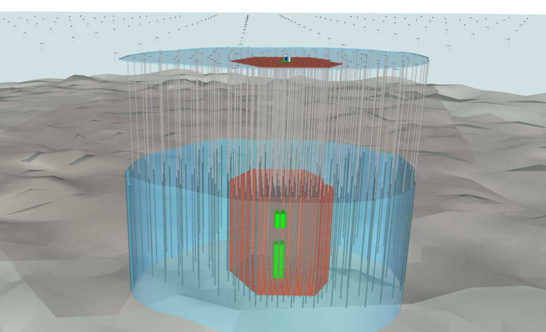
DeepCore construction begins

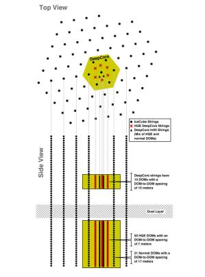
The first specialized string for DeepCore—the infill at the center of the IceCube array consisting of eight more densely deployed strings of modules—was successfully deployed in January 2009. DeepCore substantially enhanced the detector’s sensitivity at low energies: The amount of light produced when a neutrino interacts is proportional to the neutrino energy, so spacing the light sensors closer together allows the fainter low-energy events to be seen.

DeepCore started acquiring physics data in April 2010, and in May 2010, it made its first observation. DeepCore is vital for observations of lower-energy neutrinos used to investigate neutrino properties such as oscillations and searches for additional types of neutrinos, among other analyses.

Read more here, here, and here.

IceCube construction is completed

After seven seasons of construction, the final string was lowered into the last hole on December 18, 2010—and IceCube was complete! It was a milestone for science and was the culmination of efforts of hundreds of people around the world.

Read more here and here.

The first fully instrumented physics run, IC86, begins

Though IceCube had been taking data since 2005, it didn’t begin full operations until May 13, 2011, when the detector took its first set of data as a completed instrument. This is known as a “physics run.” Since then, IceCube has collected data continuously.

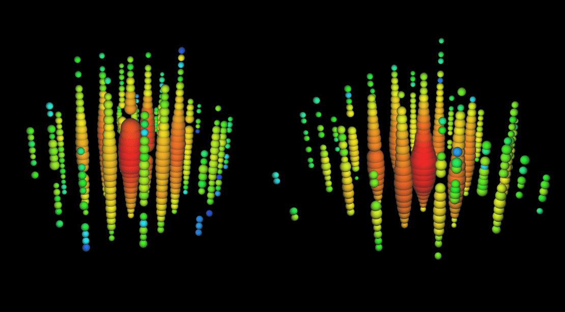
Paper is published announcing the discovery of two PeV-energy neutrinos, indicating an astrophysical neutrino flux

In May 2012, the IceCube group at Chiba University in Japan discovered two PeV-energy neutrinos in the data from the past year. One, nicknamed “Bert,” had been detected in the IceCube array in August 2011; the other, “Ernie,” had been captured in January 2012. While not statistically significant enough to claim a first observation of astrophysical neutrinos (2.8 sigma), the two events were a first indication of an astrophysical neutrino flux. The results were published on July 8, 2013, in Physical Review Letters. Read more here and here.

IceCube results show strong evidence for an astrophysical neutrino flux

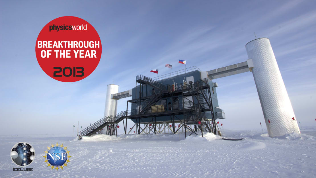
In November 2013, the IceCube Collaboration announced the discovery of 26 astrophysical neutrinos in addition to Bert and Ernie—significantly more than background expectations. With energies between 30 and 1,200 TeV, these neutrinos were the most energetic ever observed. And though their flavors, directions, and energies were inconsistent with what we would expect from neutrinos produced in Earth’s atmosphere, they did match predictions for neutrinos of extraterrestrial origin. Together, these detections showed strong evidence for an astrophysical neutrino flux. The results were published in Science.

This discovery heralded the beginning of the exploration of the universe with neutrino telescopes and would later be named “Breakthrough of the Year” by Physics World.

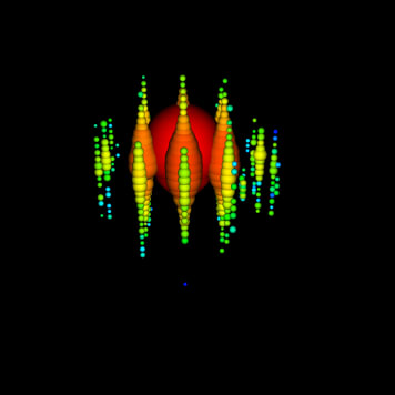
IceCube announces the discovery of the highest energy neutrino at the time

On September 2, 2014, the IceCube Collaboration published a paper in Physical Review Letters describing the detection of the highest energy neutrino ever observed at the time. The 2-PeV event was nicknamed Big Bird.

IceCube confirms cosmic neutrino flux with muon neutrinos traversing Earth

In a paper published on August 20, 2015, IceCube confirmed its 2013 astrophysical neutrino flux results with an independent analysis of neutrinos that had come mostly from the northern sky. Since IceCube is located at the South Pole, searching just the northern sky allowed IceCube to use Earth as a filter against cosmic-ray muons, which, unlike neutrinos, cannot travel all the way through the planet.

From this analysis, IceCube detected 21 neutrinos above 100 TeV, which could not be explained by neutrinos produced in Earth’s atmosphere and were most likely astrophysical in nature.

Read more here and here.

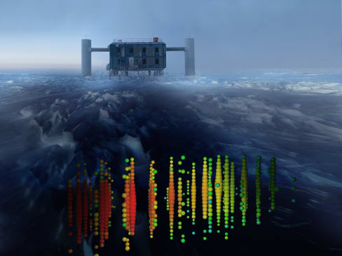
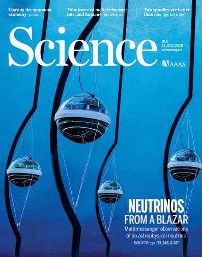
Science papers describe first source of high-energy neutrinos by the first successful multimessenger campaign involving neutrinos

Two papers published in Science on July 12, 2018, provided the first evidence for a known blazar as a source of high-energy neutrinos detected by IceCube. This blazar, designated by astronomers as TXS 0506+056, was singled out following a neutrino alert sent by IceCube on September 22, 2017. IceCube broadcast coordinates of that alert to telescopes worldwide for follow-up observations. Gamma-ray observatories, including NASA’s orbiting Fermi Gamma-ray Space Telescope and the Major Atmospheric Gamma Imaging Cherenkov Telescope (MAGIC) in the Canary Islands, detected a flare of high-energy gamma rays associated with TXS 0506+056, a convergence of observations that convincingly implicated the blazar as the most likely source. Read more here, here, and here.

NSF approves funding of the IceCube Upgrade

On June 25, 2019, NSF approved full funding to upgrade the IceCube detector, significantly extending its scientific capabilities to lower energies and improving the fidelity of past and future data through better ice measurements. The IceCube Upgrade project will introduce seven strings of optical modules at the bottom center of the 86 existing strings, adding more than 700 new and enhanced optical modules to the 5,160 sensors already embedded in the ice beneath the geographic South Pole.

Read more here.

This side-by-side comparison of a simulated muon neutrino event shows how the IceCube Upgrade will be able to detect events of lower energies than the current detector. Credit: IceCube Collaboration

IceCube submits white paper outlining plans for IceCube-Gen2, the next-level extension of the detector

The IceCube Neutrino Observatory is performing admirably, but to make new physics discoveries and continue to probe the mysteries of the universe, a bigger and more sensitive detector is needed.

So, in August 2020, the international IceCube-Gen2 Collaboration submitted a white paper that outlined the need for and design of a next-generation extension of IceCube. By adding new optical and radio instruments to the existing detector, IceCube-Gen2 will increase the annual rate of cosmic neutrino observations by an order of magnitude, and its sensitivity to point sources will increase to five times that of IceCube.

Read more here.

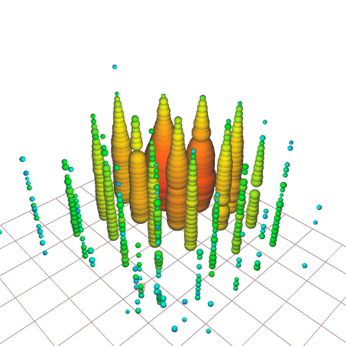
Nature paper describes IceCube’s detection of a 6.3-PeV neutrino via the Glashow resonance

On December 8, 2016, a high-energy electron antineutrino hurtled to Earth from outer space at close to the speed of light carrying 6.3 PeV of energy. Deep inside the ice sheet at the South Pole, it smashed into an electron and produced a particle that quickly decayed into a shower of secondary particles. IceCube had seen a Glashow resonance event, a phenomenon predicted by Nobel laureate Sheldon Glashow in 1960. With this detection, scientists provided another confirmation of the Standard Model of particle physics. It also further demonstrated the ability of IceCube to do fundamental physics. The results were published in Nature on March 10, 2021.

Read more here and here.