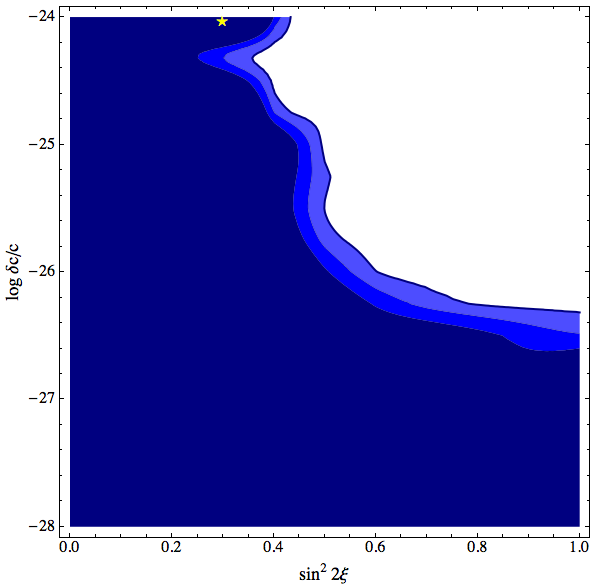
Figure 7.1: Allowed regions (90%, 95%, and 99% CL) and best fit point (marked with star) in VLI parameter space (velocity splitting and mixing angle) assuming no new physics (one MC test); EPS version
John Kelley, UW-Madison, May 2008
We have tested the analysis methodology by calculating our sensitivity to each of our hypotheses given that the null hypothesis is true. Specifically, we take one Monte Carlo sample drawn from the predicted Bartol flux with no new physics and run it through the analysis as if it were data. The results are shown in the following figures:
Figure 7.1: Allowed regions (90%, 95%, and 99% CL) and best fit point (marked with star) in VLI parameter space (velocity splitting and mixing angle) assuming no new physics (one MC test); EPS version
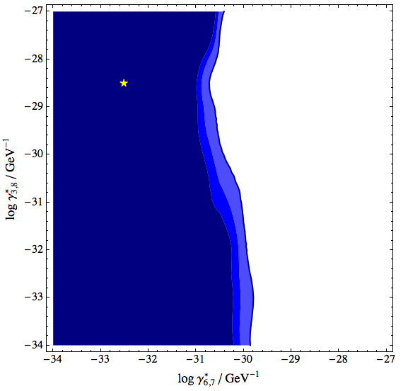
Figure 7.2: Allowed regions (90%, 95%, and 99% CL) and best fit point (marked with star) in QD parameter space (decoherence thresholds) assuming no new physics (one MC test); EPS version
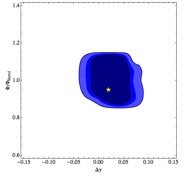
Figure 7.3: Allowed regions (90%, 95%, and 99% CL) and best fit point (marked with star) in conventional parameter space (norm. and change in spectral index) assuming a Bartol spectrum (one MC test); EPS version
We can also present the result of the conventional analysis as a band of allowed energy spectra defined by the envelope of curves representing the 90% confidence level boundary in figure 7.3. The energy range in such a plot is taken as the 5%-95% region in MC (we conservatively marginalize over OM sensitivity when finding that region).
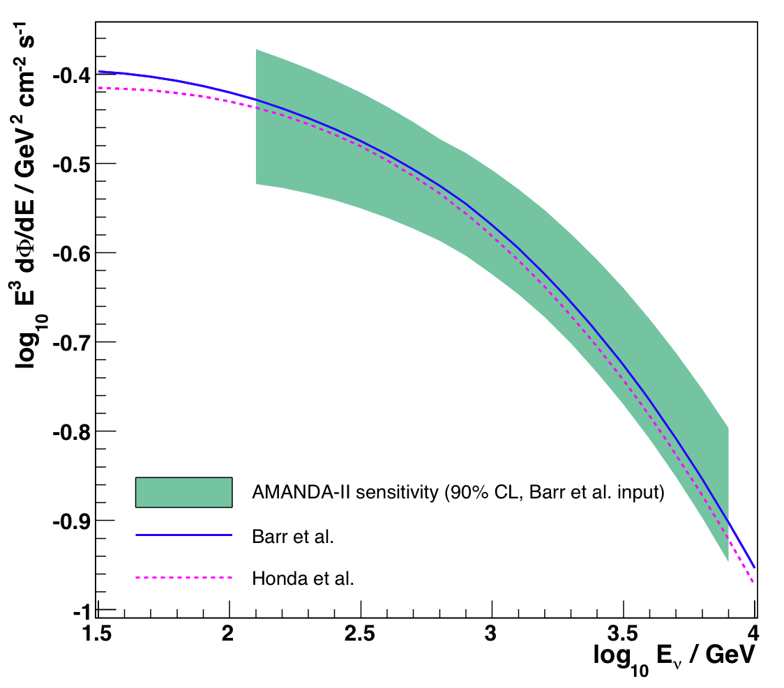
Figure 7.4: Integral hemispherical flux (upgoing nu_mu + nu_mu_bar), allowed spectra compared to Bartol and Honda 2006 predictions (one MC test); EPS version