
Figure 9.1: VLI survival probability as a function of energy, for delta_c/c = 1e-26 and two baselines.
John Kelley, UW-Madison, May 2008
No. The "central" prediction for the null hypothesis is a Bartol spectrum with OM sensitivity scaled by 85%, and then the uncertainty in the normalization (+/-20% in the NP case) is applied when minimizing the likelihood. For the conventional analysis, we will find acceptance regions for both Honda2006 and Bartol MC inputs as a consistency check of the method.
Because using it is more powerful than not. The likelihood minimization will "normalize" the MC to the data if it is within the uncertainty range; however, in the case of large new physics parameters, the deficit in nu_mu may be over 50%, meaning we can easily exclude these hypotheses even with our uncertainty in the absolute flux.
These have been added to the data page. The possible cuts on these two variables are loose compared to the space angle cut.
These have been added to the simulation page.
After the unblinding proposal was released, I found a few effective ways to isolate the remaining background contamination in the Zeuthen sample without resorting to the Nch distribution, so an additional purity cut has been added before unblinding, and the unblinding procedure has been simplified.
First, I wanted to use a three-flavor model, since to me the most "natural" case was flavor-agnostic and would result in with a 1:1:1 flavor ratio, and a 2/3 loss of nu_mu (instead of 1/2 in the two-family model). The Gago et al. work is the only full description of this that I know of.
Then, one has to choose how to deal with the four gammas. The simplest case is setting all the gammas to be equal -- this reduces to a single exponential decay term and is comparable to the simplest two-flavor models, just with a limiting survival probability of 1/3 instead of 1/2. But I could handle a bit more complexity than this, so I chose to group the four gammas into two groups based on how they appear in the survival probability.
There is no reason other than simplicity. As a test, I reduced the number of cos(zenith) bins while keeping the number of Nchannel bins equal to 10. The sensitivity got worse monotonically (but nonlinearly) with fewer bins, which is to be expected, since by reducing the number of bins one always loses information.
One nice thing about the profile likelihood method is that one does not need to choose a PDF for the nuisance parameters -- only a range of allowed values. Each nuisance parameter is another "axis" in the likelihood space, and you just minimize the likelihood with respect to all of them. You still are just using a product of Poisson probabilities over the bins of your observable when calculating the likelihood at each point in parameter space. That's because at each point, you've already specified all the physics parameters and all the nuisance parameters to be a particular value -- do you don't need to vary the nuisance parameters with a PDF any more. The variation is accomplished with the likelihood minimization search.
I have added a brief description of each study on the systematics page.
In most cases I simulated two extreme cases and used this as the uncertainty estimate for that particular source of error. In the likelihood method, though, I also use intermediate points when searching through the four combined-error nuisance parameter space.
In the systematic errors, I did
estimate the contribution from
nu_mu -(oscillate)-> nu_tau -(interact)-> tau -(decay)-> muon
This is already pretty small (~2%) because you lose energy in the tau decay and
the input spectrum is (approximately) a steep power law. Other effects,
such as
nu_mu -(oscillate)-> nu_tau -(interact)-> tau -(decay)-> nu_mu -(interact)-> muon
are much smaller because you need two interactions instead of one, and we are operating in the energy range (< 10 TeV) where interaction probability in the Earth is still small.
After the purity cuts, we estimate it to be less than 1% via a cut-tightening ratio procedure and then add it as a systematic error on the normalization.
This is a factor by which I linearly scale all the cut variables in the "tighter" or "looser" direction. A more thorough explanation has been added to the data section.
For the conventional atmospheric analysis, I want to measure the normalization and the change in spectral slope of the atmospheric flux. So in the likelihood methodology, these become the "physics parameters" with which I characterize my hypotheses, and the other systematic errors are still marginalized as nuisance parameters.
I do still have a nuisance normalization parameter (of +/-10%). But this is necessary -- otherwise, we're saying we have no error on the measurement of our normalization on the atmospheric flux. What I do is to try and measure the flux normalization while retaining the other sources of error (such as cross section) which would affect our measurement.
Keen observation! This is because the vertical events at Nch ~ 120 are in the second survival probability maximum (no chance of oscillation) for this particular value of delta_c/c (1e-26). If you look at figure 5.7, you can see that the median energy for Nch ~ 120 is around 10 TeV. Now, see the following figure which shows the survival probability as a function of energy for two different baselines (veritical, and zenith = 150 degrees) -- one can see that the oscillation maximum for the events off the vertical is pushed to higher energy, and thus more of them oscillate away.
Figure 9.1: VLI survival probability as a function of energy, for delta_c/c = 1e-26 and two baselines.
The actual situation is even more complicated, though, because the Nch/energy correlation is likely a function of zenith angle. If we could actually measure the energy reasonably well, we could trace the minima:
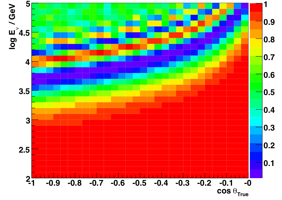
Figure 9.2: Ratio of VLI (delta_c/c = 1E-26) to conventional flux, true energy vs. true cos(Zenith), 2000-2006 atmospheric neutrino MC.
The two main differences are:
For the combined errors / nuisance parameters, since there is no PDF (and in particular, it's not Gaussian), there isn't a way to define a "sigma." One is only saying: "I believe this error covers the range of possibilities." For the individual errors, we generally still have no idea what the PDF looks like, so again there's no concept of "sigma."
The coverage properties of the method are not guaranteed; using the profile likelihood is an approximation, and there are possibly pathological cases in which one could conceivable get some undercoverage. However, all examined cases in the literature report excellent coverage properties.
That said, we can test the coverage properties using the simple case of Poissonian signal + background. Here we assume some true signal mean mu and background mean b, but in the C.L. construction we only assume a range of b around the true value, [b_low, b_high]. We then perform an "experiment" as if we were doing an analysis, construct the confidence belt given N_obs, and check if mu lies within the belt. By doing this many times we can measure the coverage of the method.
We first run a test with fixed background nuisance parameter (in which the profile construction method limits to the normal Feldman-Cousins construction) to verify coverage, which should be correct by construction. Then we examine the coverage for different true values of the background spanning the nuisance parameter range. The results are shown in the table below. We find that while there is some overcoverage if the nuisance parameter is in the middle of the range, the coverage properties are good even for extreme values of the nuisance parameters and match the desired C.L. to the precision of this test.
| Background | Coverage at 90% CL |
| Fixed (FC) | 89.5% |
| Low end of range | 89.5% |
| Middle of range | 93.1% |
| High end of range | 89.5% |
Table
9.1 Results of coverage test for profile construction on
Poisson signal+background.
For this test, mu = 8, and the background
range was [0,3].
We also show the distributions of the likelihood ratio and confidence level as a function of mu for one particular experiment where N_obs = 12. The 90% CL extracted from figure 9.4 of (4.0, 16.0) matches the tables in Feldman-Cousins for N_obs = 12 and b = 3.
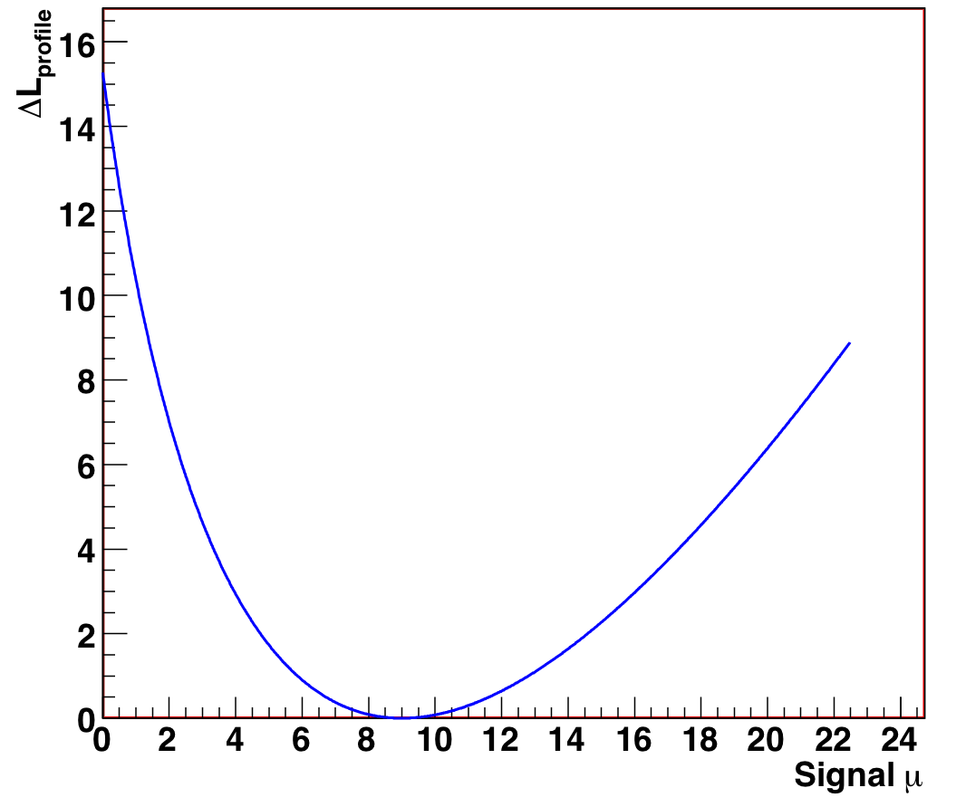
Figure 9.3: Standard likelihood ratio as a function of signal mean mu, for N_obs = 12, known background = 3 (mu_true = 8). |
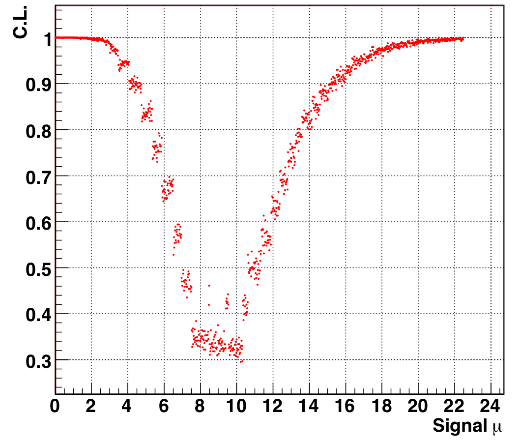
Figure 9.4: Confidence level as a function of signal mean mu, for N_obs = 12, known background = 3 (mu_true = 8). The 90% allowed region is the band of mu for which CL(mu) < 0.9. |
When one then allows the background to float as a nuisance parameter from [0,3] the 90% CL changes to approximately (5.0, 17.3), as shown in figure 9.6. The upper range expands due to the increased systematic error, as we would expect. The fact that the lower bound does not actually increase exposes the overcoverage of the original Feldman-Cousins construction due to Poissonian discreteness, which is broken by the inclusion of a nuisance parameter. This quirk is discussed by Feldman in his talk at PHYSTAT05 but is not really relevant to our analysis.
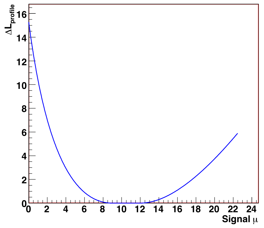
Figure 9.5: Profile likelihood ratio as a function of signal mean mu, for N_obs = 12, background range [0,3] (mu_true = 8, b_true = 3). |
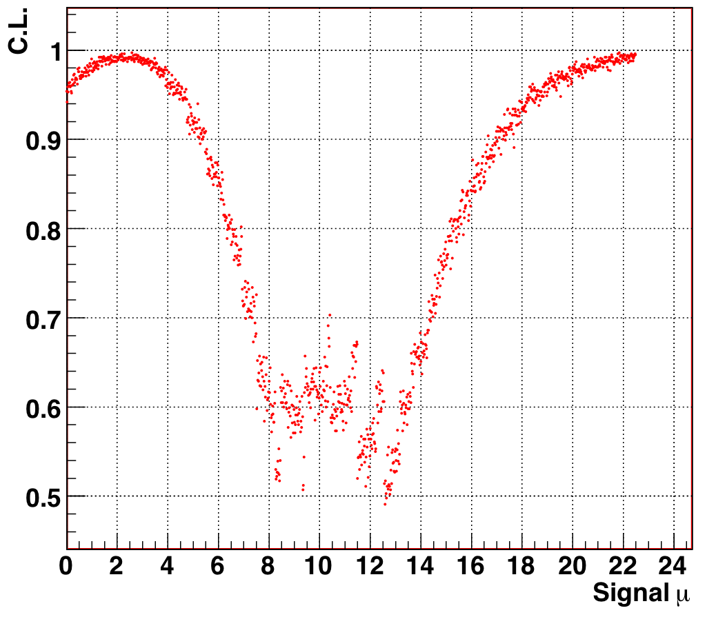
Figure 9.6: Confidence level as a function of signal mean mu, for N_obs = 12, background range [0,3] (mu_true = 8, b_true = 3). The 90% allowed region is the band of mu for which CL(mu) < 0.9. |
Because the excess does not fit any new physics signal hypothesis we are testing, leaving the excess in the data sample without changing anything means either 1) we are incorrectly modeling the atmospheric neutrino flux, or 2) we have incorrectly modeled our background contamination (as Nch-independent). In both cases the limits we calculate will be incorrect. In the conventional analysis, leaving the excess in is a statement of belief that they are truly atmospheric neutrinos, in which case the results would suggest the spectrum is significantly harder than the models predict.
This suggests that we must both address the excess and make a judgment call about what it is. Since analysis strongly suggests the excess consists of misreconstructed muons, we have made the choice to try and remove the events in an unbiased way. The other alternative is to not remove them but model the systematic error background contamination as Nchannel-dependent, but for this one would still need to quantify the excess -- a procedure that has the same dangers.
The new Nch-dependent cuts do tighten the condition on the JAMS-Pandel space angle, but our original cuts on LdirB and NdirC were pretty loose. The excess does show up in "poor" half of both these distributions (increasing confidence that they are background), but unfortunately simply cutting out the excess region would remove a lot of atmospheric neutrinos as well. Fortunately, we find that after the Nch-dependent cuts are applied, both distributions agree much better with atmospheric neutrino MC.
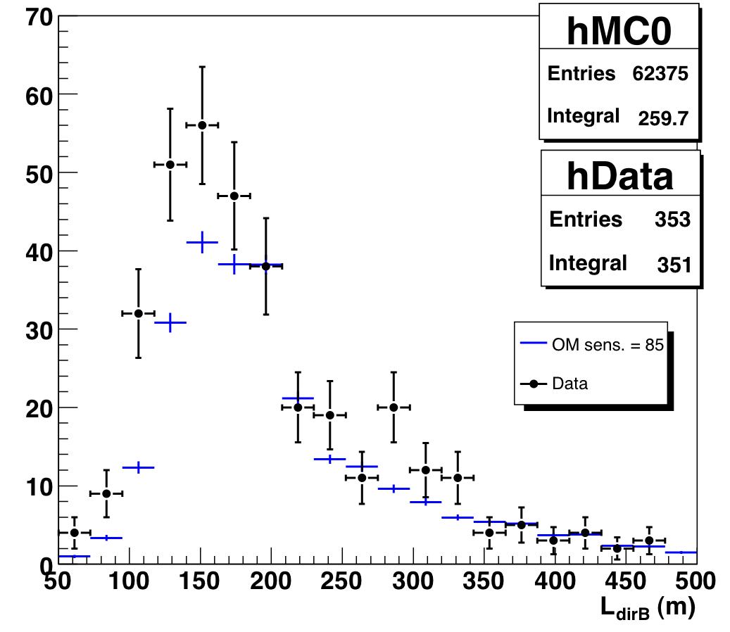
Figure 9.7a: Direct length of data and atmospheric neutrino MC, Nch > 65. |
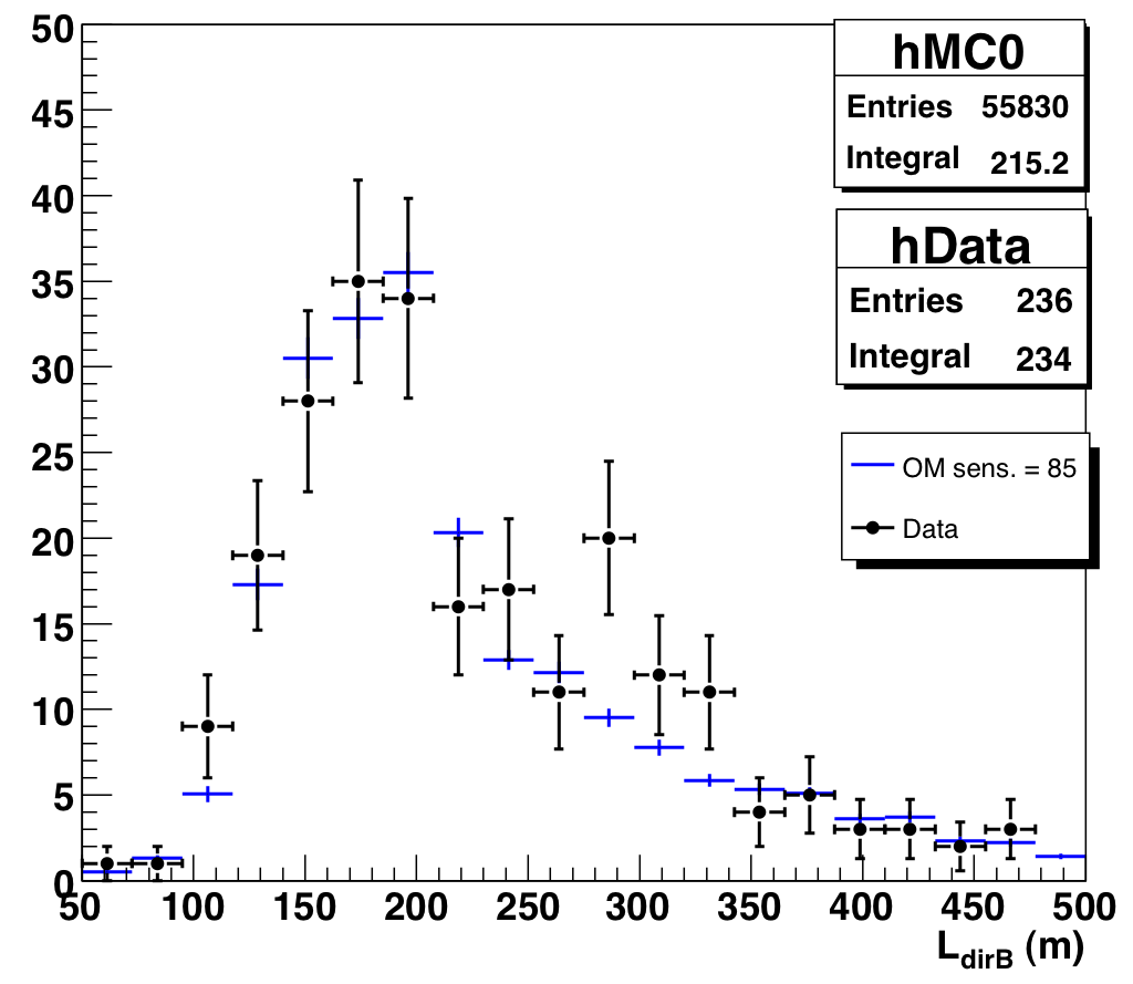
Figure 9.7b: Direct length of data and atmospheric MC, Nch > 65, after new Nch-dependent cuts. |
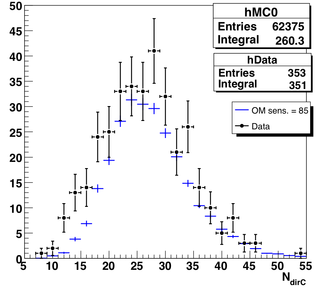
Figure 9.8a: Number of direct hits of data and atmospheric neutrino MC, Nch > 65. |
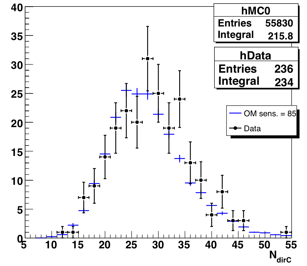
Figure 9.8b: Number of direct hits for data and atmospheric neutrino MC, Nch > 65, after new Nch-dependent cuts. |
No. Because only O(1%) of MC atmospheric neutrino events are removed, the median sensitivity is not affected (log delta_c/c = -26.4 before and after for VLI).