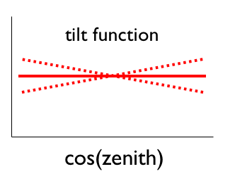
Figure 6.1: Schematic illustrating the linear cos(zenith) tilt parameter.
John Kelley, UW-Madison, May 2008
As described in the analysis methodology, systematic errors must be quantified and incorporated into the likelihood analysis at an early stage. Furthermore, cannot only consider systematic effects that change the normalization of our atmospheric flux prediction; we must also model uncertainties that could change the shape of the zenith angle or Nch distributions.
We have thus split the systematic errors into four classes, depending on their effect on our observables:
The following table lists all the systematic errors that have been incorporated into the likelihood analysis, along with which of the above four classes to which they belong.
Error |
Type |
Size |
How |
Atm. flux model |
norm |
+/-18% |
|
Cross section, scattering angle |
norm |
+/-8% |
|
Reconstruction bias |
norm |
-4% |
|
Nu_tau-induced muons |
norm |
+2% |
|
Background contamination |
norm |
+1% |
|
Charm contribution |
norm |
+1% |
|
Timing residuals |
norm |
+/-2% |
5-year paper |
Muon energy loss |
norm |
+/-1% |
5-year paper |
Rock density |
norm |
<0.1% |
|
Primary CR slope (incl. He) |
slope |
+/-0.03 |
|
Charm contribution (slope) |
slope |
+0.05 |
|
Pion/kaon ratio |
tilt |
+1%/-3% |
|
Charm (tilt correction) |
tilt |
-3% |
|
OM sensitivity + ice |
OM sens. |
+/-10% |
The normalization errors are added in quadrature, while the much smaller tilt and slope errors are added linearly. For any rounding necessary for the likelihood analysis (which is grid-based), we round errors up. For the NP analysis, that results in the following total errors in each class:
Error Type |
Total |
Normalization |
+/-20% |
Slope |
-0.04,+0.08 |
Tilt |
-6%,+3% |
OM sens. |
+/-10% |
We are now in a position to explain fully how the conventional analysis works: the atmospheric neutrino flux normalization and the slope terms become physics parameters instead of nuisance parameters. There is still an error on the normalization (all the other uncertainties above except the leading +/-18%), but it is smaller. The tilt and OM sensitivity errors remain the same. Thus we have the following total uncertainties for the conventional analysis:
Error Type |
Total |
Normalization |
+/-10% (flux norm. becomes physics parameter) |
Slope |
becomes physics parameter |
Tilt |
-6%,+3% |
OM sens. |
+/-10% |
The error on the atmospheric flux normalization was determined by comparing the predicted fluxes given by the Honda2006 and Bartol flux models in NeutrinoFlux. The difference in the combined event rate is only 7%; however, this masks larger differences in the predicted individual nu_mu and nu_mu_bar event rates (18% and 11% respectively). We feel that the latter was more indicative of the true uncertainty in the models, and so take +/-18% as the error on the flux normalization.
To estimate the combined error due to cross section and scattering angle, we compared our nusim-based MC with a sample generated with ANIS (which uses the more modern CTEQ5 cross-sections, and accurately simulates the neutrino-muon scattering angle). We find an 8% difference for an atmospheric neutrino spectrum. More details can be found here.
By "reconstruction bias," we mean errors caused by systematic shifts in the quality cut parameters between data and MC. Such systematic shifts occur in both paraboloid error and smoothness (see the comparisons here). To quantify this effect, we first calculate the scaling factor for each parameter which maximizes the Kolmogorov probability when comparing data and MC:
Parameter |
K-S Scaling Factor |
abs(Sphit) |
1.09 |
Perr |
1.025 |
Normally, nu-tau-induced muons are negligible when considering atmospheric neutrinos, since oscillations are such a small effect. However, in the new physics scenarios we consider here, up to 50% of our nu_mu flux can oscillate to nu_tau, which can then interact, generate a tau, and then decay to a muon. To estimate this flux, we generated a sample of tau neutrinos with ANIS. Then, we weighted each event with a nu_mu atmospheric weight times its oscillation probability, for the extreme case described above. The final event rate was only 2% of the total. The reason the flux is so small is that you are penalized by a huge factor by the steep spectrum when you consider that the muon takes only a fraction of the tau energy.
To estimate the uncertainty from neglecting any charm contribution to the atmospheric neutrino flux, we used NeutrinoFlux to compare the predicted flux when adding the Naumov RQPM flux (probably the most extreme flux still under consideration). We find the difference to be 1% at our final cut level. We also incorporate the effect on the Nch distribution by modeling the charm contribution as a tilt in the energy spectrum. We find that changing the spectral index by +0.05 matches the increase at high Nch caused by the Naumov flux. Changing the spectral index actually distorts the zenith angle spectrum by a tiny amount (3% tilt), but we saw no observable difference when just adding the Naumov flux, so just to be conservative we "correct" for this by adding in a tilt uncertainty along with the slope term described above.
The five-year paper quotes a 10% uncertainty in the density of bedrock at under the polar ice. To model the effect of this, we recompiled both ANIS and MMC, increasing the density of rock by 10% in both, and compared to an unmodified ANIS sample. We found a difference in atmospheric event rates of <0.1%. We note that increases in interaction probability due to increased density are offset by decreased muon range.
To determine the effect on the zenith angle distribution from the uncertainty in the pion/kaon ratio, we first implemented an atmospheric flux weighting scheme which directly uses the Gaisser parametrization (Cosmic Rays and Particle Physics, eq. 7.5). This is similar to what NeutrinoFlux does internally for its high-energy extrapolation. We then compared the cos(Zenith) distributions using extreme values for A_K / A_pi of 0.28 and 0.51, as derived from the Z_N-pi and Z_N-K uncertainty tabulated in Agrawal et al..
The effect is small and can be approximated by a linear tilt in the cos(zenith) distribution of +1%/-3%, where the tilt value refers to the percent change at cos(zenith) = 0. This is shown diagrammatically in figure 6.1:
Figure 6.1: Schematic illustrating the linear cos(zenith) tilt parameter.
This is similar in methodology to what J. Ahrens did in the 2000-2003 oscillation analysis (that analysis cited a SuperK thesis for the error).
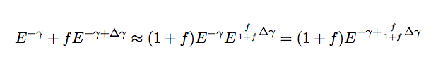
As discussed in Gaisser et al., some uncertainty remains in the primary cosmic ray spectral index. If this is small, we can model this by just changing the spectral slope by some delta_gamma. The uncertainty in the slope of the proton component is small (0.01), but the uncertainty in the Helium component is much larger (0.07). To find how much this uncertainty changes the total flux, we approximate a change in spectral index of a secondary component as follows:
Determining the range of uncertainty on the OM sensitivity, as well as its central value for the ice model used in the simulation, required a dedicated study. The Zeuthen analysis used the shape of the atmospheric neutrino zenith angle distribution to constrain the OM sensitivity (with PTD/MAM) to 100%+3%-10%. However, we cannot use this approach since this distribution is blinded; so, we have used the downgoing atmospheric muon rate to get a handle on the OM sensitivity.
The dominant error in the predicted atmospheric muon rate is the uncertainty in the hadronic interactions in the atmosphere. We model this by generating dCORSIKA events with the EPOS, SIBYLL, and QGSJET-II hadronic models, which bracket a range of predictions. We compare these rates to the rate in a subsample of 2005 data (56 Hz after basic hit- and crosstalk-cleaning). As shown in figure 6.2, the SIBYLL model at 85% OM sensitivity agrees with the data well, and using the uncertainty of the hadronic models we can estimate the OM sensitivity to within +10%/-7%.
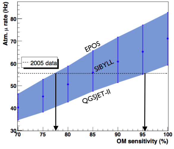
Figure 6.2: Downgoing muon rate vs. OM sensitivity, with band of predictions for various hadronic models.
We note that the range of error from this method is similar to the Zeuthen result, if a bit more conservative (17% here vs. 13%). The difference in the mean is due to the ice model. The details are beyond the scope of this proposal, but all released ice models using Photonics (Millennium, Elves, AHA) produce a much higher rate of muons and atmospheric neutrinos than the prediction by PTD/MAM. We can "fix" this discrepancy by turning down the OM sensitivity -- this is why we lump ice uncertainty in with OM sensitivity. We note that a mean sensitivity of 85% as derived from the muon analysis also pulls the neutrino prediction in line with PTD/MAM:
Ice Model |
Atm. neutrino rate vs. PTD/MAM |
Millennium |
+39% |
AHA |
+23% |
AHA (85% OMs) |
-8% |
K. Hoshina, G. Hill, and J. Lundberg are continuing investigations into Photonics and have fixed a number of bugs, but none so far address this large discrepancy.