Atmospheric Neutrino Unblinding Proposal
AMANDA-II 2000-2006
John Kelley, UW-Madison, May 2008
8. Excess
Observables
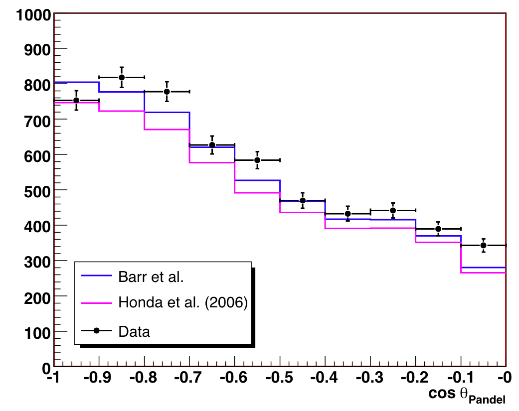
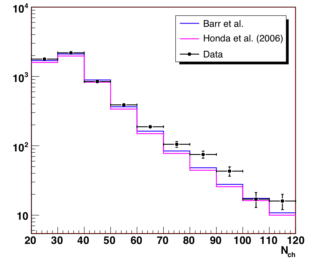
After the original unblinding, we examined the observable distributions, Nch
and cos(Zenith). The data are consistent with the predicted conventional
atmospheric neutrino flux models, with the exception of a 1.5% excess in
the (60 < Nch < 120) region. This is
slightly higher than the estimated 0.5% background contamination, and more
importantly, it is not distributed evenly across the observable space
(which is how we model background contamination in the systematic errors).
In this section, we discuss the impact of the excess, and how we have
chosen to address it.
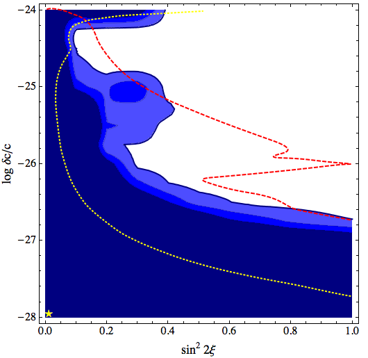
Limits on VLI and Quantum Decoherence
Initial limits on VLI (violation of Lorentz invariance) and quantum decoherence
are quite reasonable, and better than the median sensitivity, because of
the small excess at high Nch. This is because the data are less compatible
with a small new-physics signal, which would show up first as a
deficit at high Nch. Because the excess is not modeled in the systematic
errors, these limits are artifically low.
A note on the decoherence limits: the shape of the allowed region looks
different than the test sensitivity shown in figure 7.2, but this is not
necessarily unexpected. The confidence level of the region along the y-axis
is particularly sensitive to the systematic errors, and in some test cases
with MC, we see results which look qualitatively like the contours
shown above.
Constraints on the Conventional Flux
Unfortunately, the conventional analysis is significantly impacted by the
high-Nch excess. This is because the background is modeled in the
likelihood only as a uniform normalization error, not as something which is
energy-dependent. The likelihood analysis therefore models the atmospheric
flux as significantly harder (a change of spectral index of +0.1) to compensate
for the extra events. We do not believe this is a meaningful result.
Analysis of the Excess
What is the excess?
An analysis of the events in the Nch (60,120) region suggests that
the excess (about 85 events compared to MC normalized to the low-Nch
region) consists of misreconstructed muons. Salient observations about
the excess include:
- The excess is evenly spread across all years;
- Events scanned in the event viewer deemed "poor" appear non-tracklike (perhaps
muon bundles passing outside the detector) and appear preferentially
in the clean ice regions, but we did not notice other distinguishing
topologies (such as association with certain strings or OMs);
- These poor events tend to have worse up- to down-going likelihood
ratios;
- And perhaps most convincing, a significant fraction of the excess
appears to have higher paraboloid error and JAMS/Pandel space angle
difference.
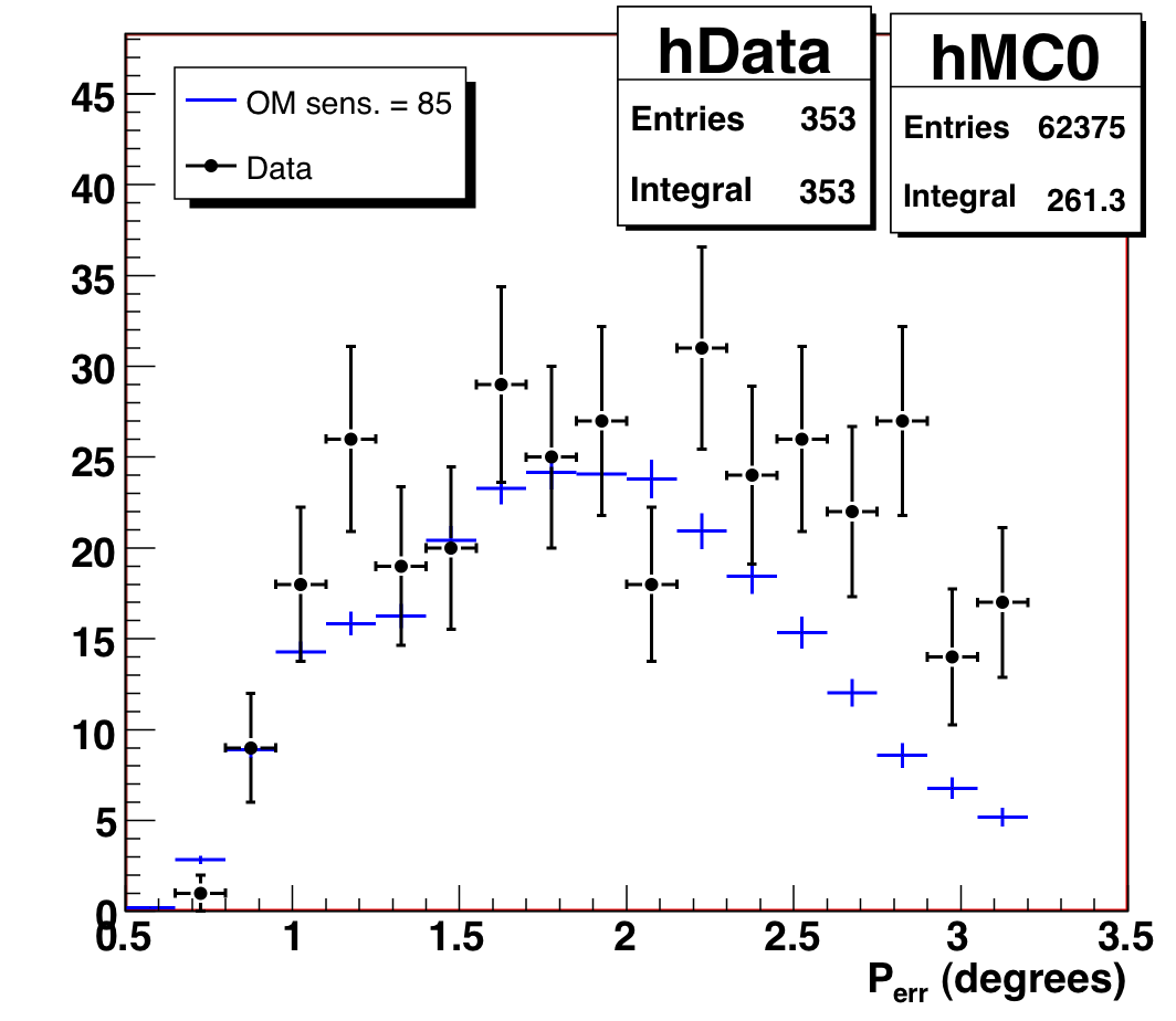
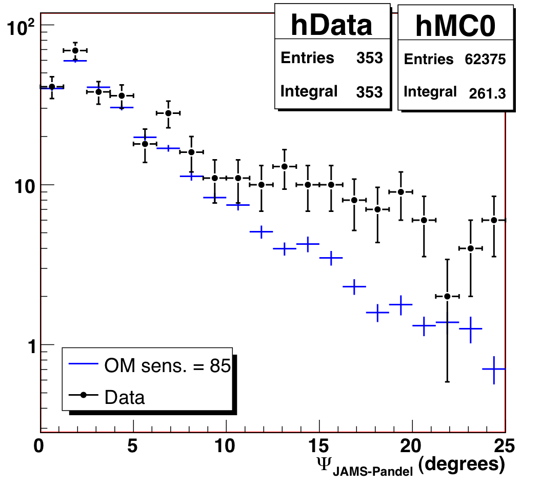
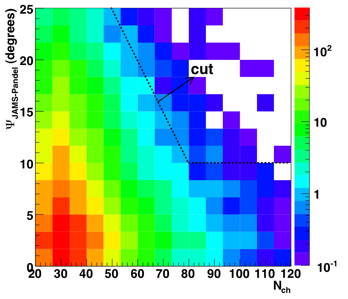
To illustrate the last point we show the distribution of paraboloid
error and JAMS/Pandel space angle for high-Nch events. Note the excess
is concentrated at poor values of both --- what one would expect for
misreconstructed background. We therefore have chosen to isolate and remove
the excess, developing a well-motivated procedure which is not biased
simply to force data-MC agreement (since we have already unblinded).
Isolating the excess
In order to isolate the excess we note another point from
the previous section: the excess is concentrated at poor up-to-down
likelihood ratio. We can therefore first roughly isolate the population
via their likelihood ratio, and only then apply any cuts to paraboloid error
and space angle difference. Instead of using a constant value we note that
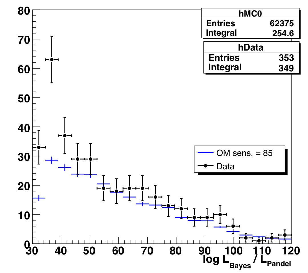
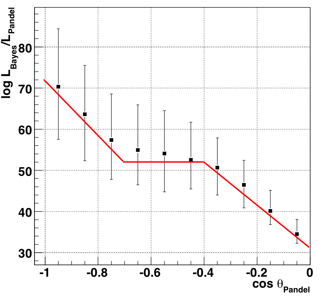
the likelihood ratio is very dependent on the zenith angle, so instead we
follow the median LR as a function of cos(zenith), as derived from MC.
To reiterate what we are doing: we perform this as a first selection on
which to then apply Nch-dependent cuts on the other quality variables.
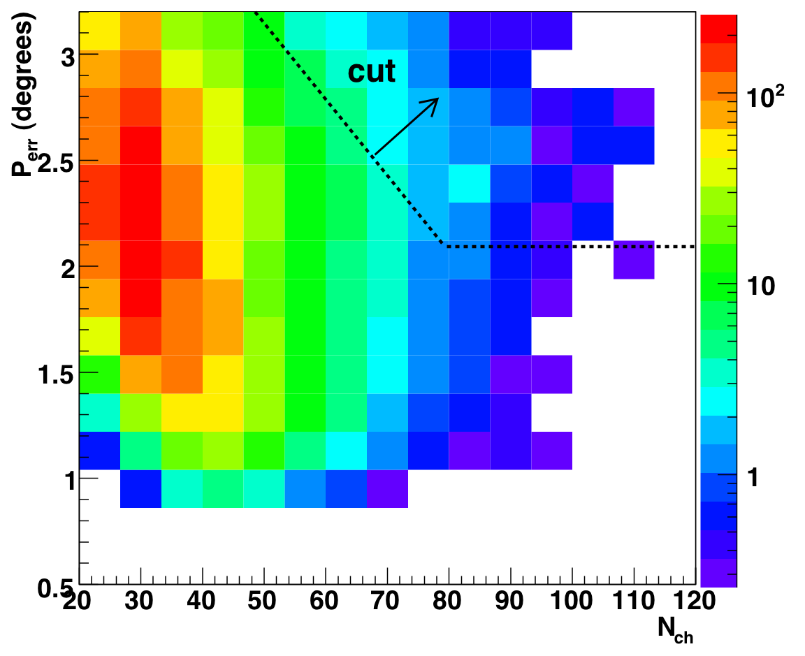
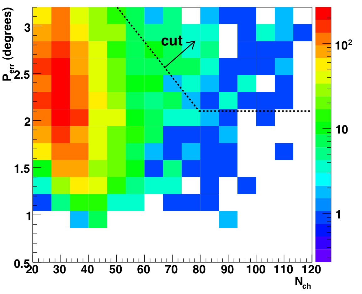
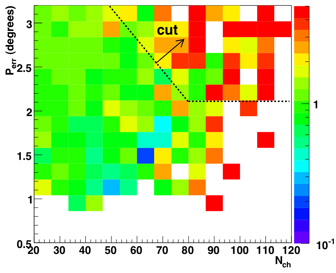
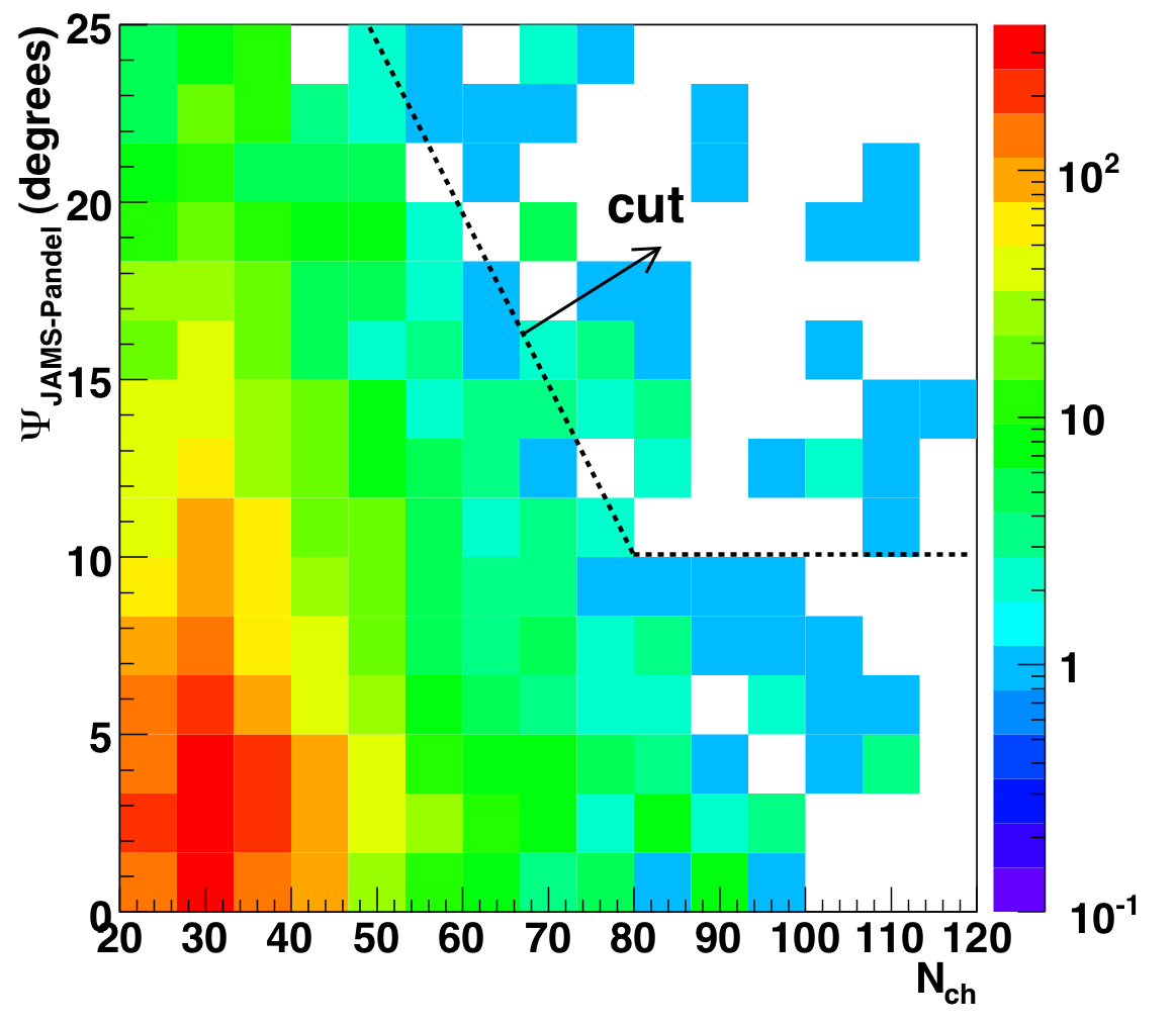
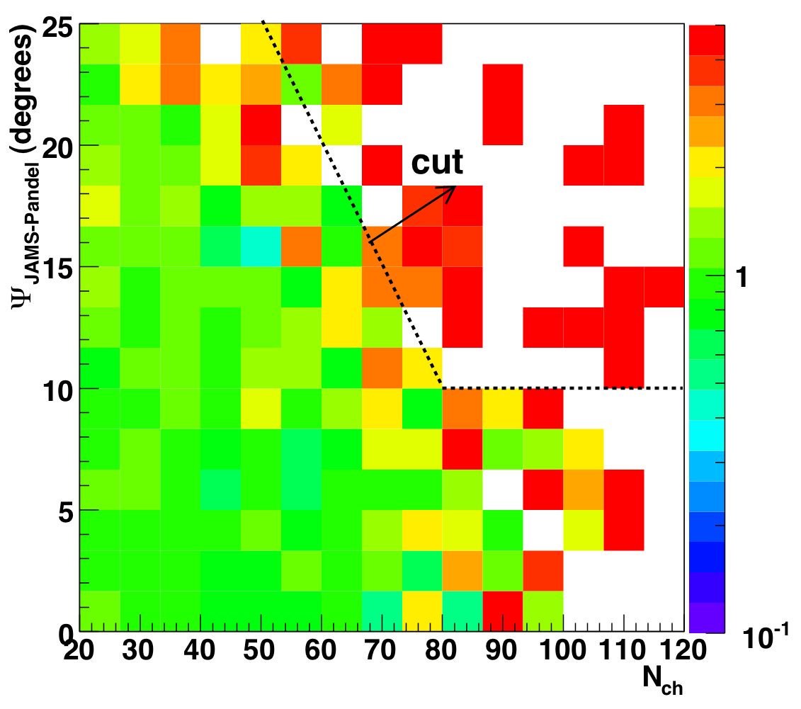
To determine how to tighten the cuts as a function of Nch, we examine 2D
plots of paraboloid error and space angle vs. Nch, only for the events
below LR_median(theta) (see figure 8.7b). A 2D cut is shown superimposed on the
distributions for atmospheric MC (left), data (center), and the ratio of
data to MC (right).
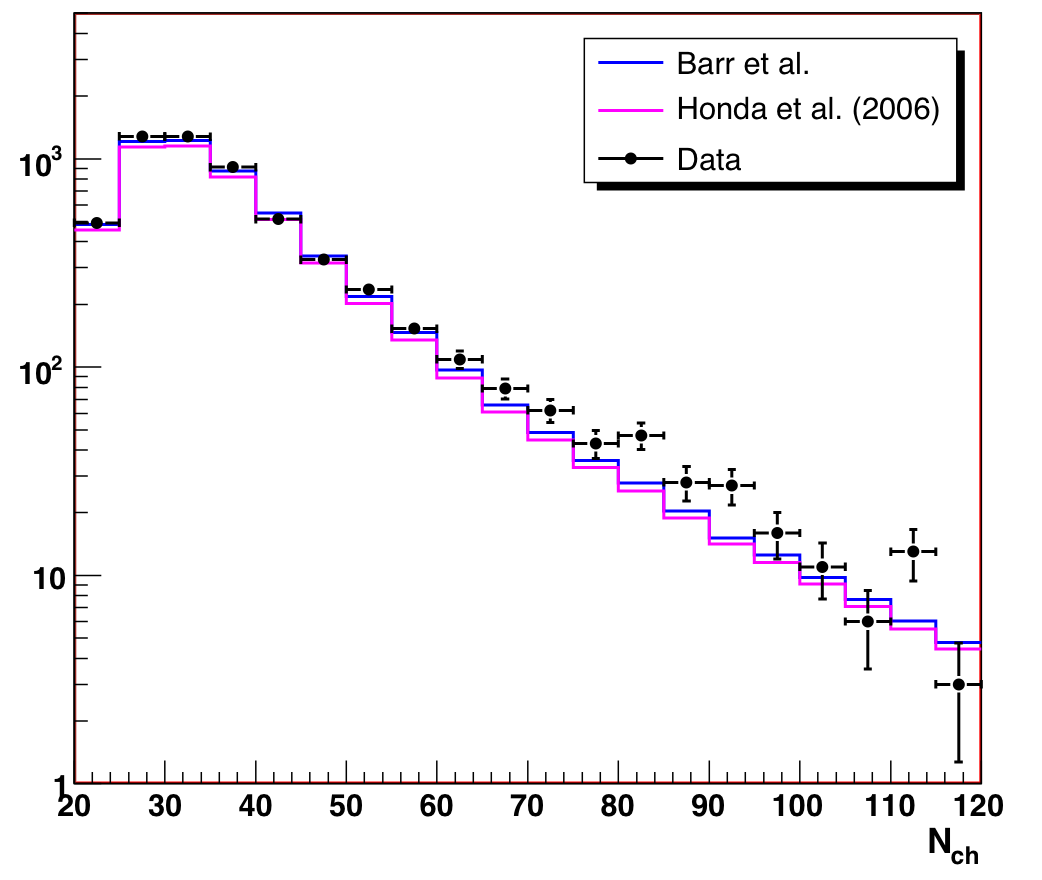
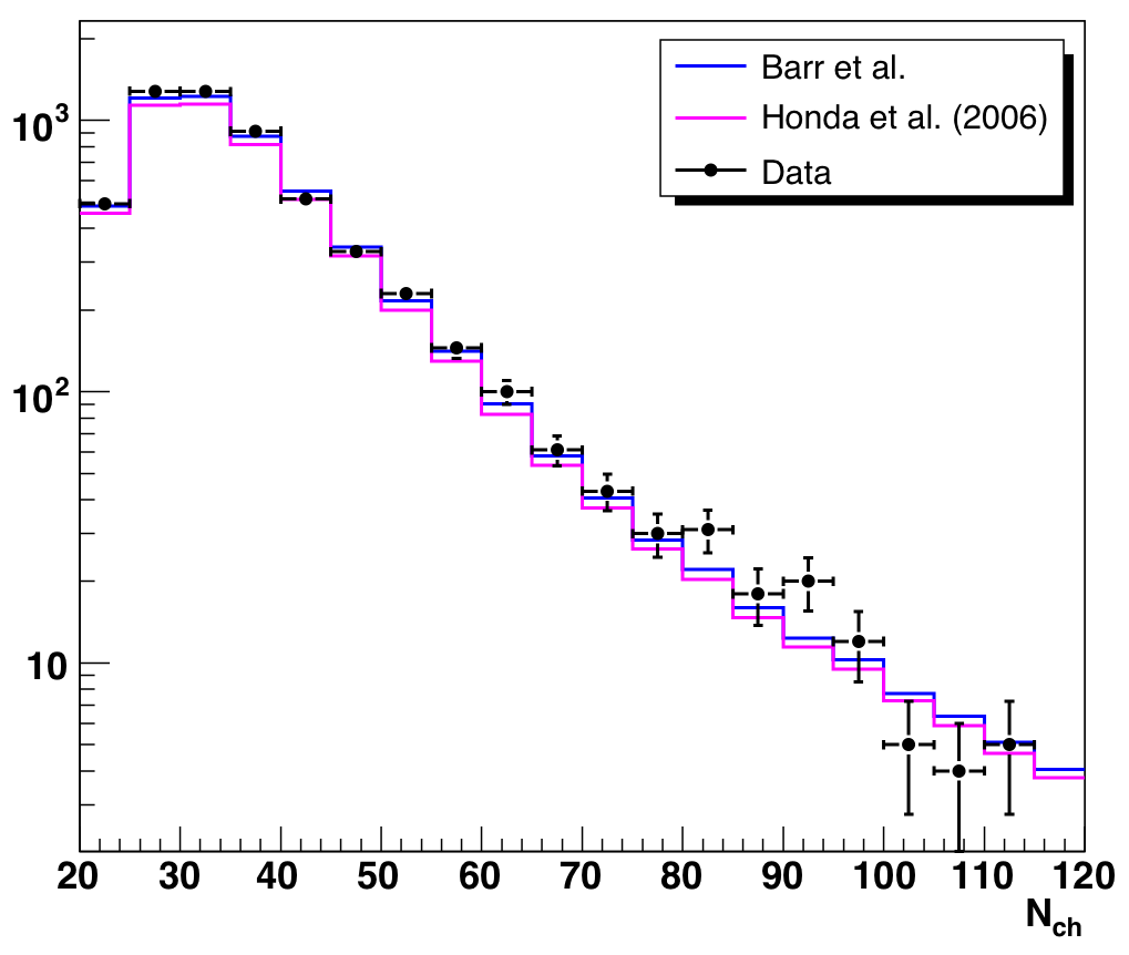
Applying these test cuts reduces the data in the analysis region from 5638
to 5511 events (-2.3%), while reducing the (not normalized) atmospheric MC from
5399 to 5341 events (-1.1%). After applying these cuts, the agreement in
the Nch distribution is significantly improved, with little loss in
sensitivity to atmospheric neutrinos.
Although we designed the cuts to be zenith-agnostic, we find that most of
the events removed are more horizontal than vertical. The small number of
events removed does not, however, appreciably change the zenith angle
distribution.
As a note, we had previously posted an event we considered bad because
it was not tracklike: event 2166924
(Quicktime MOV
or AVI). After designing these cuts
we noted that this event is one of those removed. In general, we note a
high correlation with randomly selected, high-Nch events classified by eye as
questionable (in the event viewer) and the events removed by the 2D cuts.
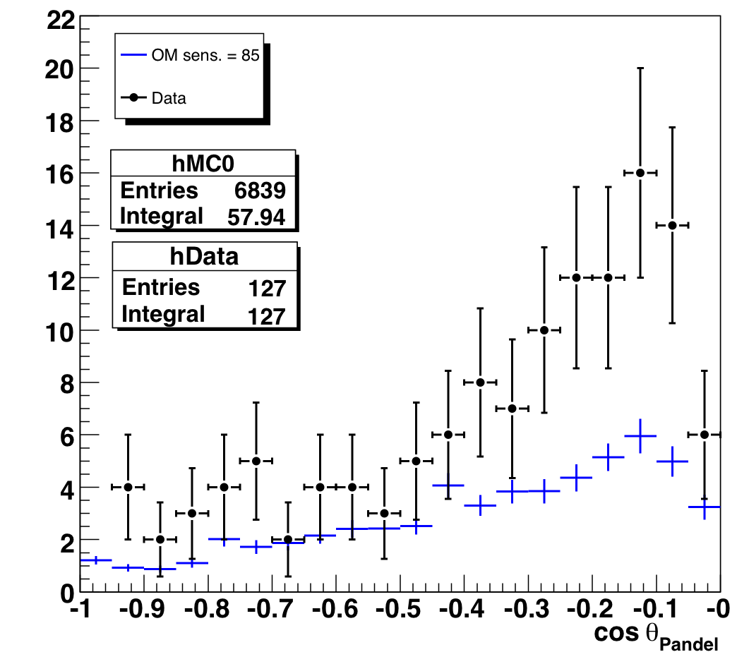
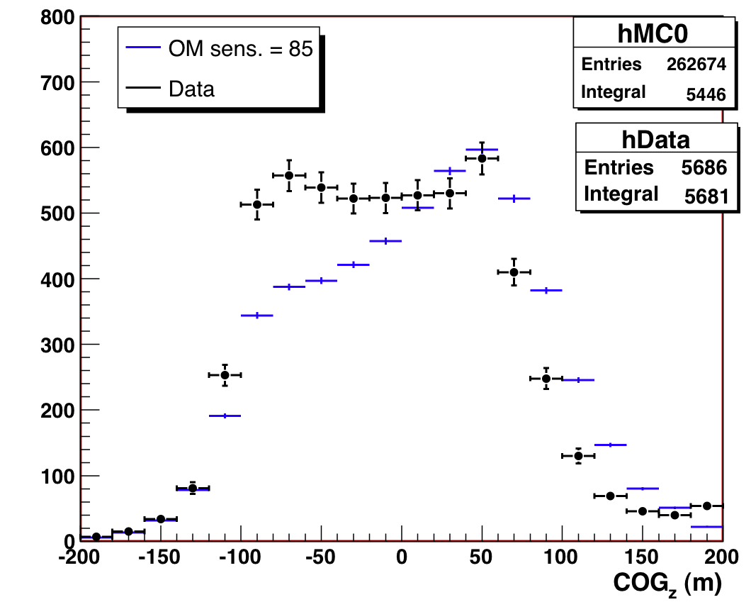
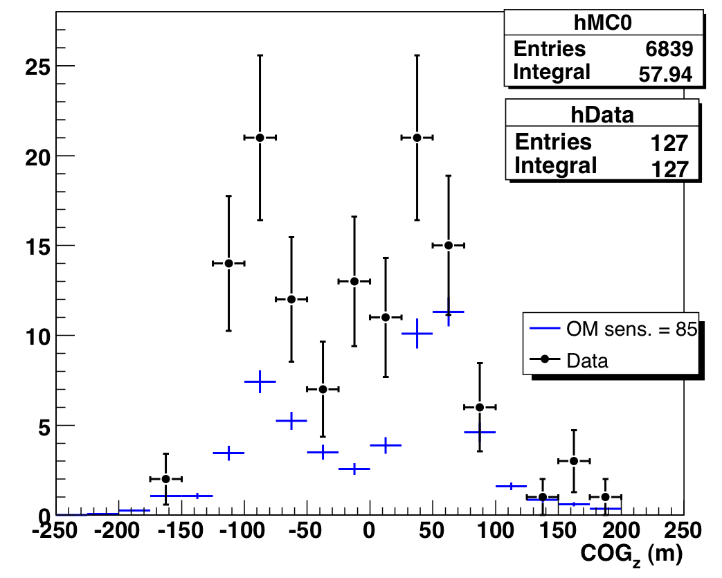
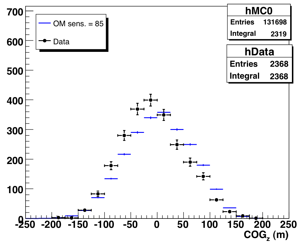
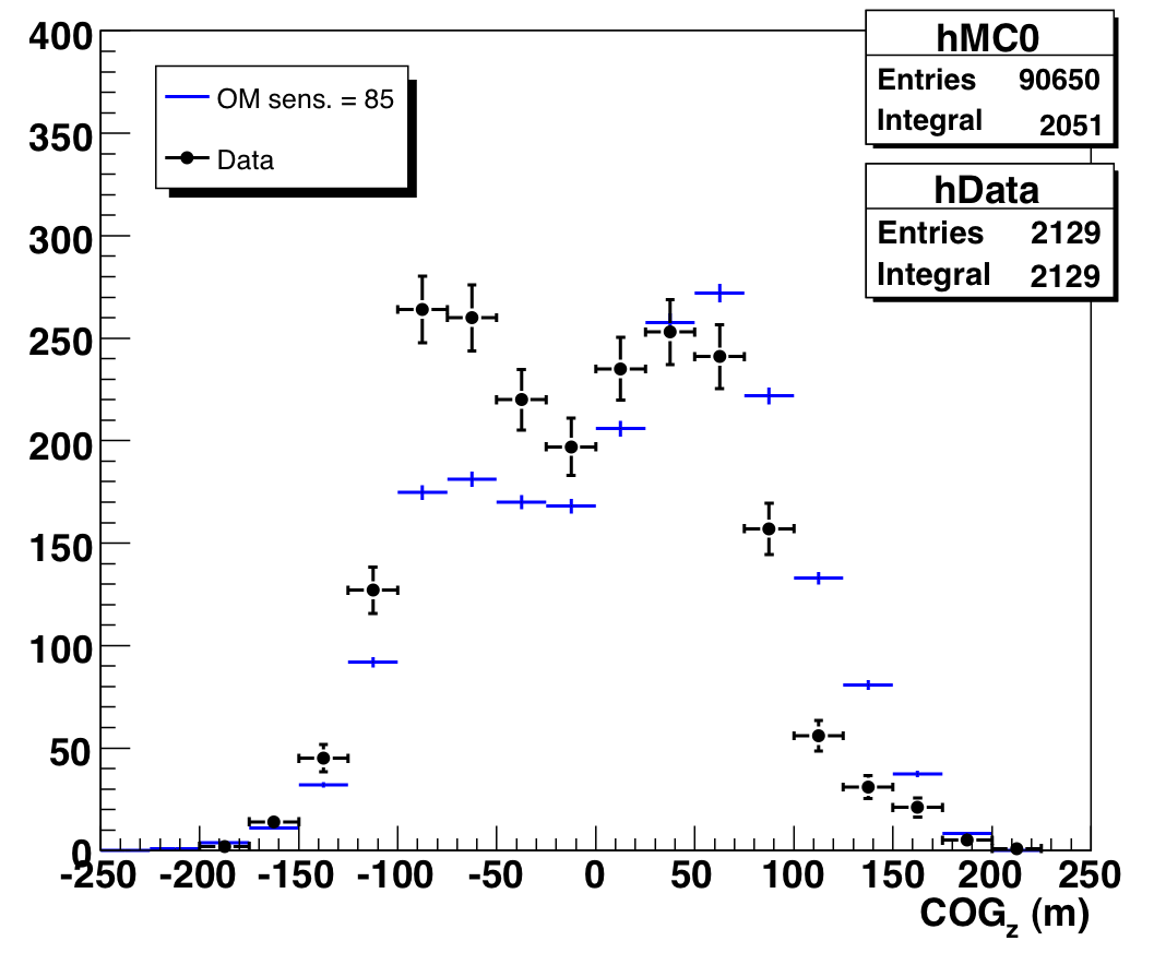
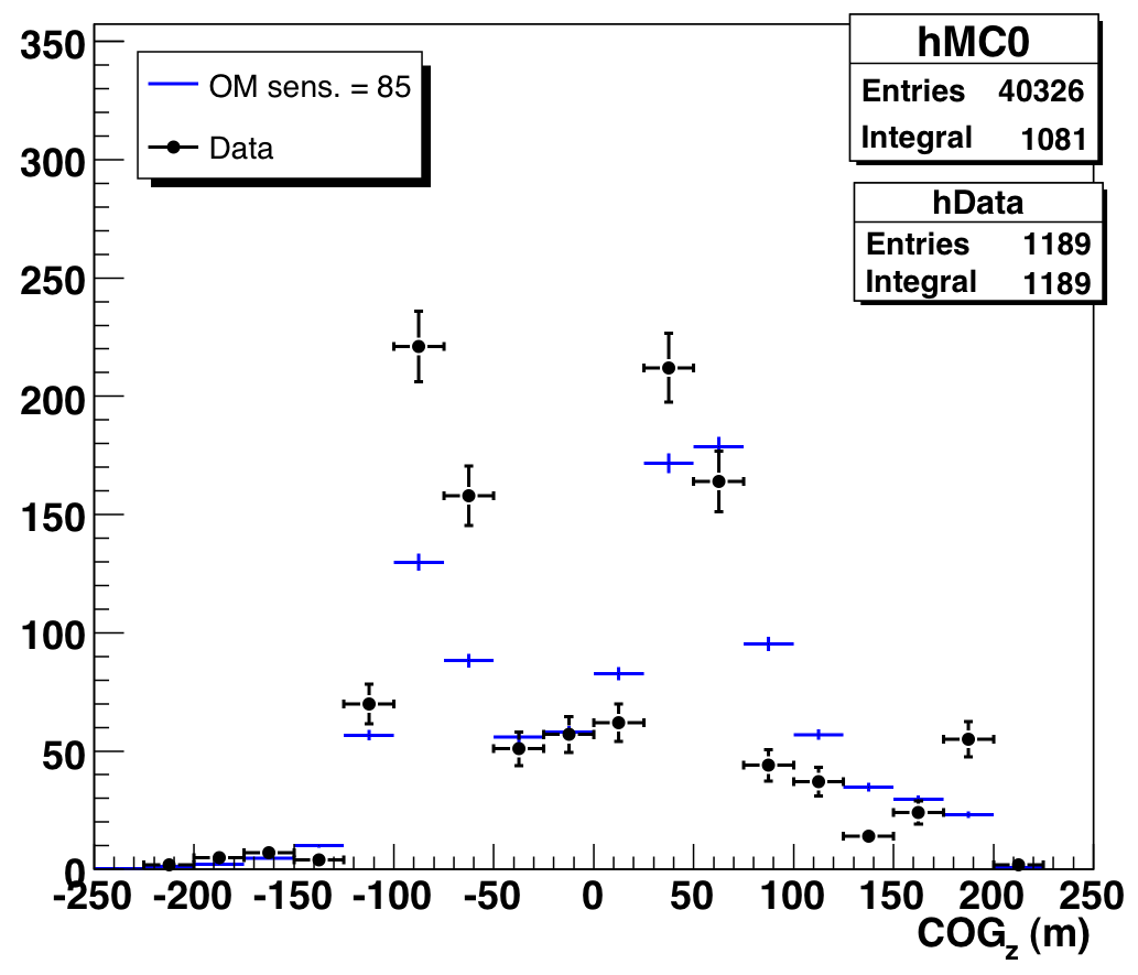
A Note on COGz
There is also an excess in the COGz peaks: however, the COGz structure
over the whole sample is not well-reproduced by the simulation. We feel it
not unreasonable that just as in level 3 data, misreconstructed
muons at this high purity level are more likely to show up in the COGz peaks.
We also show the COGz distribution for various zenith angle ranges
(before the Nch-dependent purity cuts described above -- distributions
look the same after the cuts):
The differences between data and MC in the rightmost plot (horizontal
events that are primarily probing one ice layer) mirror the discrepancies
found in
our ice model
timing residual analysis.
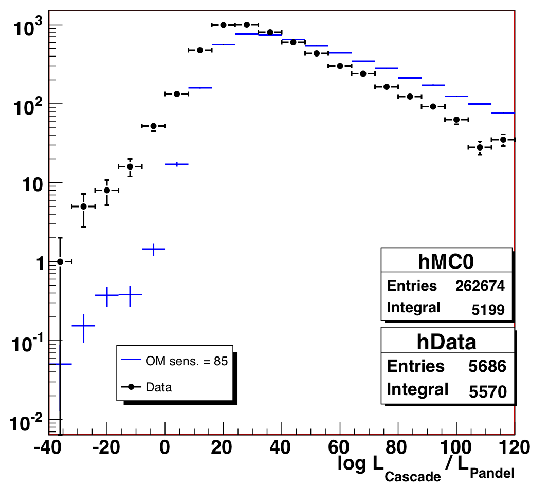
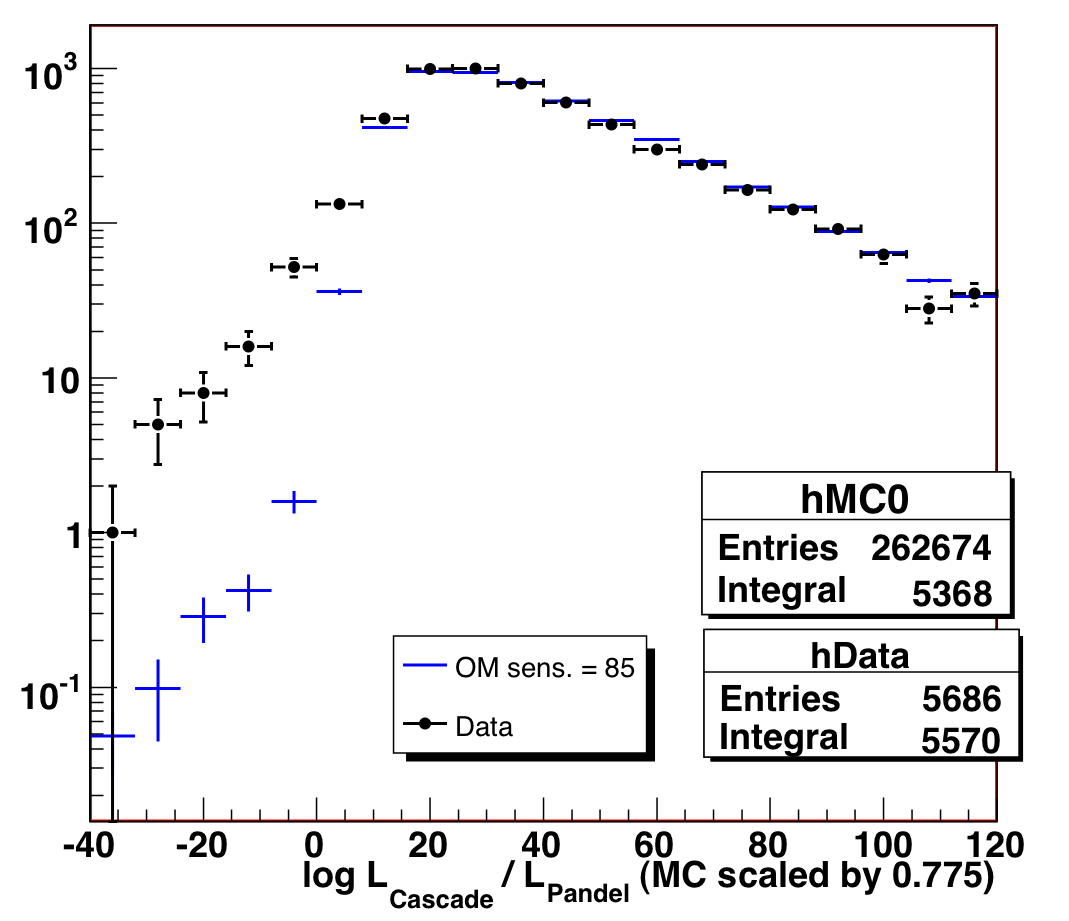
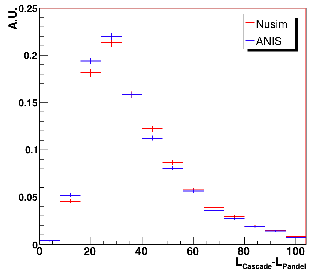
A Note on the Cascade Likelihood Ratio
As part of this investigation, we seriously considered using the
cascade-to-track likelihood ratio as a cut parameter, as many of the
questionable events are not very tracklike. However, this variable is not
well-reproduced in MC. If we scale the MC variable by a factor of 0.775
(determined via Kolmogorov test), the distribution agrees much better, but
there is a still an excess in the data at low values (less tracklike). We
were not comfortable that this excess was truly misreconstructed background
to remove it. We mention it here for completeness and as a avenue of
further investigation -- if it is background, this could be another 3% of
contamination that is undetectable by the existing cuts described here.
It is also possible that understanding the MC scaling factor could lead
to insights about the ice model.
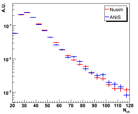
Alternate Hypotheses
One other hypothesis that we have examined and rejected is that the events are
misreconstructed neutral current cascades that are not simulated in our
nusim MC. While there is a clear excess of cascade-like events in ANIS L3
relative to nusim, this does not really persist to the final cut
level, and the Nch distributions are nearly identical: