
IceCube Detector Overview
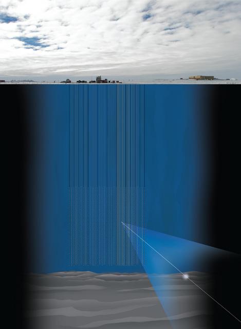
Fig. 1, IceCube Detector
IceCube is a cubic kilometer neutrino telescope buried beneath roughly 1.5 km of ice at the geographic South Pole. The size of the detector will allow scientists to detect neutrinos at a higher resolution and with more accuracy than similar neutrino telescopes of this type. IceCube is the largest detector built of this type in the world (see Fig. 1). IceCube's predecessor, the Antarctic Muon and Neutrino Detector Array (AMANDA), was the proof of concept for IceCube. The detector itself is being constructed deep within the ice using a hot water drill. Approximately 4,800 Digital Optical Modules (DOMs), or photomultiplier tubes, are inserted into the ice on 80 cables referred to as "strings." Each string holds 60 DOMs. Although IceCube is currently a work in progress with 40 strings successfully deployed into the ice, the detector will be completed in 2011.
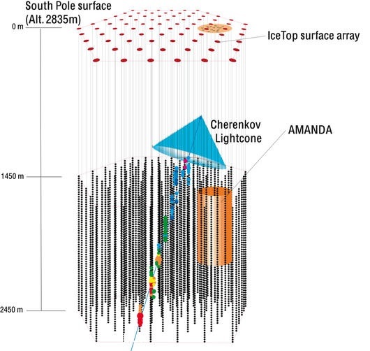
Fig. 2, IceCube Event
IceCube works on the principle of Cherenkov light. The DOMs are able to detect the faint light given off by high energy particles when they travel faster than the speed of light in the ice (similar to a sonic boom), as shown in Fig. 2. The goal of the detector is to identify high energy neutrinos (from 10^11 to 10^18 eV). However, the neutrinos cannot be detected directly. Instead, they are detected when neutrinos interact with atoms in the ice, producing muons. Nevertheless, cosmic rays impacting the atmosphere produce showers of particles, including pions and kaons that decay into muons, which provide a large amount of background for the detector. "Downgoing" refers to muons that enter the detector from above the horizon (0 to 90 degrees) and "upgoing" refers to muons that enter the detector from below the horizon (90 to 180 degrees), in which the zenith is zero. There are approximately a million downgoing events for every upgoing event.
IceCube is able to eliminate the cosmic showers effect by using the Earth to filter out muons associated with other particles. This works because neutrinos interact very little with the surrounding particles and can travel long distances without interaction. Muons cannot travel as far because they interact frequently with their surroundings and lose energy quickly, often stopping before or in the IceCube detector itself. In this way, IceCube can successfully separate the muons from neutrinos. With this knowledge, IceCube hopes to reconstruct the tracks the neutrinos leave in the ice to galactic or extragalctic sources, such as a supernova remnants, gamma ray bursts, or active galactic nuclei (AGN).
IceCube Project Overview
The goal of my project is to analyze the IceCube-22 (IC-22) data alongside the Monte Carlo simulation data to see how they are comparable. This acts as calibration for the IceCube detector and is the first time it has been done for both the AMANDA and IceCube projects. I will do this by applying two separate levels of quality cuts--a light cut and a hard cut--to the simulation data. These cuts will help to eliminate the muons that are misreconstructed as downgoing, because, in the actual IceCube data, it will interfere with the neutrino data. These cuts will then be applied to the IC-22 data and further analyzed. Looking ahead, this analysis can be used to produce plots for further calibration, such as the muon rate flux as a function of both zenith angle and depth into the ice (Fig. 3 and 4 [1]).
 Fig. 3, AMANDA-II Muon Flux Rate as a function of Zenith Angle |
 Fig. 4, AMANDA-II Muon Flux Rate as a function of Depth into the Ice |
Quality Cuts & Event Simulation
Definition of Parameters
Zenith Angle: The angle at which the muon traveled into the IceCube detector, with respect to the vertical.
Zenith Error: The difference between the reconstructed and true track for an event in the zenith angle.
Number of Hits: This is the record of the amount of DOMs that register a hit during an event.
Direct Hit: A direct hit defines the number of DOMs in which the expected time and actual time (due to scattering in the ice) it registers a hit is less than 75 nanoseconds during an event.
Split Psi: The Split Psi is the angular difference between two split tracks.
Direct Length: The distance between the first and last DOMs in a direct hit in the IceCube detector in the occurrence of an event.
Reduced Likelihood: The reduced likelihood is fundamentally an average of the product of a group of probabilities divided by the degrees of freedom. This is used in relation to the IceCube detector to predict the parameters of a given event when the outcome is known. A more thorough approach to likelihood functions can be found here. The following equation is used to find the reduced likelihood:

 is the total probability for particular hits occurring, during an event, for a given track. The track has 5 quantifiable dimensions in which
 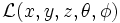 .
.
Fig. 5, Sigma Paraboloid Origins
Sigma Parab: The sigma paraboloid is a measure of the error, or standard deviation, of a track during an event. This can be obtained from plotting the likelihood function, as shown in Fig. 5 [2].
The error ellipse is useful for determining the confidence level (or standard deviation) of the track during an event. The standard deviation, sigma, is found through a paraboloid fit. The error ellipse is essentially an ellipse with two measurable standard deviations from the length and width, which translate to error in the azimuth and zenith angles. For this project, however, only the error in the zenith will be used.
Track Smoothness: The smoothness is a measure of how balanced the number of DOM hits is on a track during an event. It is measured on a scale from -1 to 1, in which -1 indicates all of hits towards the end of the track (an extreme), 1 indicates all of hits towards the beginning of the track, and 0 indicates a balance between the number of hits at the beginning and end of the track.
Initial Quality Cuts
The goal of the initial quality cuts is to improve the angular resolution of the IceCube Minimum Bias Simulation data by making cuts that will minimize the angular error while keeping a high efficiency with the data.
Useful Variables
Using IceCube simulation data, I found the correlation factors between separate variables in order to find out which variables had the most effect on one another. The zenith angle was examined in Fig. 6-8 and the variables were viewed with the zenith angle in Fig. 9-11. High degrees of correlation to the zenith error (Fig. 12-14) indicate the parameters that would lend the most quality to a cut. High degrees of correlation between two of the quality parameters shows a redundancy (Fig. 15-17), meaning they will not have a big effect on the other variables. The Direct Length, Reduced Likelihood, and Sigma Paraboloid had the highest degrees of correlation with the zenith error, or angular resolution. The plots that indicate this correlation appear smeared in a linear fashion.
 Fig. 6, Zenith Angle vs. Zenith Error |
 Fig. 7, True Zenith Angle vs. Zenith Error |
 Fig. 8, Reconstructed Zenith Angle vs. True Zenith Angle |
 Fig. 9, Zenith Angle vs. Direct Length |
 Fig. 10, Zenith Angle vs. Reduced Likelihood |
 Fig. 11, Zenith Angle vs. Sigma Parab |
 Fig. 12, Direct Length vs. Zenith Error |
 Fig. 13, Reduced Likelihood vs. Zenith Error |
 Fig. 14, Sigma Parab vs. Zenith Error |
 Fig. 11, Direct Length vs. Sigma Parab |
 Fig. 12, Direct Length vs. Reduced Likelihood |
 Fig. 14, Reduced Likelihood vs. Sigma Parab |
From this information, quality cuts can be made with the now identified quality variables to keep the most relevant data, which will refine the overall statistics of the data in terms of angular resolution.
Optimization
In making a quality cut, determining which variable leads to the highest level of optimization is the first step. This cut will be made first because it will improve the angular resolution most. The optimization was found with the following equation:

This equation was used to improve the angular resolution of the data. E_cut refers to the efficiency of the data set. E_cut is equivalent to the number of entries after the cuts divided by the number of events before the cuts. A positive consequence in doing this is that it eliminates the background (misreconstructed) data, especially close to and below the horizon. The square root of the number of entries is divided by the median of the distribution of the angular error (essentially, the position of the middle of the highest peak) in order to improve the angular resolution of the data. The most improved, or best, angular resolution is at smaller numbers. Through this process, the overall amount of data is reduced, but the overall quality of the data is predominately of a higher quality. This procedure ensures that the data has been optimized.
Cut Parameters
The highest point of optimization and the resulting cut values are shown in the following chart for each variable that indicated high levels of correlation towards the angular resolution. A Gaussian fit was applied to each variable to determine the position of the peak and number of entries contained in each peak on Fig. 23. Sigma Zenith has a high level of optimization compared to Direct Length and Reduced Likelihood because it keeps the largest amount of entries with the best angular resolution. Sigma Zenith, Direct Length, and Reduced Likelihood are optimized alone and then together, to show the level of optimization each variable has alone, and then combined (Fig. 18-22).
 Fig. 18, Sigma Zenith (alone) |
 Fig. 19, Direct Length (alone) |
 Fig. 20, Reduced Likelihood (alone) |
 Fig. 21, Direct Length (with Sigma Zenith) |
 Fig. 22, Reduced Likelihood (with Sigma Zenith and Direct Length) |
The peak's position in the graphs indicates the best place to make the cut, because it is at its most optimal. However, even though the quality cut variables do have a great effect on one another because of the redundancy, the influence is still evident. This can be seen when the cuts are made in a sequential order (with the highest level of optimization for the first cut). When optimized with Sigma Zenith, the Direct Length's peak changes position and the same can be said for the Reduced Likelihood. Thus, to obtain the best possible cut parameters, the cuts should be made when the variables are optimized sequentially instead of apart. The table below lists the cut parameters chosen. The Number of Hits is included as a general measure to ensure that the events in the simulation data have at least 8 DOM triggers (the definition of an event).
| Optimization Variable | Cut Parameter |
| Sigma Zenith | <.03 |
| Direct Length | >200 m |
| Reduced Likelihood | <11 |
| Number of Hits | >7 |
The result of making the cuts can be seen in Fig. 23. The minimum cut is defined as the number of direct hits greater than or equal to two and the degrees of freedom for the paraboloid fit not equal to zero; it is very basic of cuts to ensure overall quality in the data. There are three main parts to the structure of the cuts. The first noticeable part of the graph is the evidence that the peak shifts to the left, through each consecutive cut. When the peak moves further left, the angular resolution of the data is actually improving. Thus, the goal of the initial cuts has been achieved.
The second part of the graph is the observable decrease in the height of the peaks. This is an acceptable consequence of improving the angular resolution. However, the third main part is represented with another, smaller peak past the horizon (or the far right of the graph). There is a clear decrease in the number of muons. This represents the background, or misreconstructed, muons. These need to be eliminated so the atmospheric muons do not get confused with the upgoing muons from neutrinos; although the neutrino muons were not taken into account at this stage, the atmospheric muons need to be eliminated at angles greater than the horizon so that, in the experimental data, the misreconstructed muons do not get confused with the upgoing neutrino muons.
In all, the initial cuts provided an increase in the angular resolution of the data at the expense of the quantity of the data. However, the quality of the data is more significant that the quantity, so this is an acceptable consequence to the data.
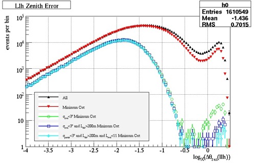
Fig. 23, Zenith Error (with cuts)
The results of the cuts can also be seen below, in Fig. 24 and 25. The angular resolution (on the y-axis) has been improved. Also noticeable is the significant reduction in the misreconstructed muons past the horizon (the smear across the top of the graphs). The horizon is located at 1.57 or Pi/2 on the x-axis.
|
Fig. 24, Zenith Error |
Fig. 25, Zenith Error (with cuts) |
The good and bad events can be judged by their angle dependence. A good event is an event which has been reconstructed with minimal error; alternatively, a bad event is an event which has been misreconstructed. The misreconstructed events that take place near the horizon are of concern because they may overpower the good events. In Fig. 26 and 27, the single muon showers can be analyzed to see the ratio of good events to bad events. This is accomplished by dividing the data into two sections--the good and the bad. Looking back to Fig. 23, the dividing line between the correctly constructed and background (misreconstructed) muons takes place at about 18 degrees (or -0.5 with the log scaling). This parameter was used the cut the data into the good and bad events. The ratio between them was found and compared in the following graphs before and after the initial cuts were made.
 Fig. 26, Zenith Angle (no cuts) |
 Fig. 27, Zenith Angle (with cuts) |
As shown, before the cuts, the bad events overpowered the good events, especially below 70 degrees (0.2), but afterwards there were significantly less bad events close to and below the horizon.
Angular Resolution
The following is a study of the Zenith Resolution of the IceCube detector as a function of Zenith Angle (done with and without quality cuts). The angular resolution can be gauged in two separate ways: the first is how good the angular resolution is (or how low the red line appears on the graph), the second method is used to see the consistency of the angular resolution (essentially, the flatter the slope of the line is, the more consistent the angular resolution is). The angular resolution improved drastically after the cuts (Fig. 28 and 29). Thus, the initial cuts were successful.
 Fig. 28, Angular Resolution (before cuts) |
 Fig. 29, Angular Resolution (after cuts) |
Final Quality Cuts
The goal of the final quality cuts is to eliminate the misreconstructed muons close to and beyond the horizon with the IceCube Muon Filtered Simulation data through the use of quality cuts.
Single vs. Coincident Muons
Single muon showers are events in which there is one recorded track going through the IceCube detector at a given time. Coincident muon showers are events in which there are two separate tracks of muons going through the IceCube detector at the same time. Coincident muon events compose roughly 5% of the total muons events. The difficult part in analyzing coincident muon events comes from separating one track from another and reconstructing the tracks and angles at which the muons entered the detector. Additionally, the coincident tracks may also look like a single track, which provides a greater difficulty in the reconstruction.

Fig. 30, Coincident Muon Simulation Data Cases
The Muon Filtered Simulation data for the coincident muons, however, is particular because it saves only the data for one of the tracks. In doing so, there are three cases that arise (as shown in Fig. 30).
In Case #1, the simulation data saves the reconstructed track with the correct true track. On the left, the black arrows represent the true track while the red lines represent the reconstructed tracks. Case #1 results in the smallest angular error. This is the most frequent case.
In Case #2, the simulation data saves the reconstructed track with the wrong true track. In doing so, this results in the largest angular error. However, both the reconstructed track and the true track are still good data separately. Thus, the data obtained in case #2 is still acceptable.
In Case #3, the simulation data completely misreconstructs the muon tracks. This is the case that provides incorrect data and must be eliminated through the use of cuts.
The percentage of single muon versus coincident muons can be viewed in Fig. 31 and 32. The graphs (and corresponding data sets) are normalized to the same rate. In this particular case, the data is normalized in relation to time. By normalizing the data, the events can be compared on the same time scale, eliminating any discrepancies in the data due to the time difference.
 Fig. 31, Single vs. Coincident Muons |
 Fig. 32, Single vs. Coincident Muons (log) |
In Fig. 32, the case of the coincident muon can be seen visually. In the first peak, the coincident muons follow the curve of the single muons--this is case #1. At ten degrees (1), the single muons drop off, while the coincident muons form a second peak--these are the muons in case #2. Lastly, at 90 degrees (2), or the horizon, the third case of the muons is exhibited. These muons are the misreconstructed muons that need to be eliminated and the reason the final quality cuts are necessary.
Fig. 33, Ratio of Coincident Muons to Single Muons
As further evidence of the need for the final cuts, the ratio of the coincident and single muons was taken after the first cut (Fig. 33), clearly showing a dominance of coincident muons close to and past the horizon (90 degrees).
Background Suppression
To eliminate the misreconstructed muons entirely, more cut variables were assessed to see if they would make quality cuts. This was done by viewing each variable against the angular resolution with the coincident muon filtered simulation data and distinguishing the features, or cases, of the coincident muon to determine the position of case #3 and the parameter needed to eliminate it. Fig. 34-37 are examples of the cut parameters chosen and the effect on the variable before and after the cut.
 Fig. 34, Direct Hits vs. Angular Resolution (before cuts) |
 Fig. 35, Direct Hits vs. Angular Resolution (after cuts) |
In viewing the number of direct hits, the three cases are visible. The first case the furthest left, the second near the middle, and the third is represented in the vertical smear on the right side. As shown, this vertical smear has been completely eliminated with a hard cut. The same reasoning can be applied to the Track Smoothness.
 Fig. 36, Track Smoothness vs. Angular Resolution (before cuts) |
 Fig. 37, Track Smoothness vs. Angular Resolution (after cuts) |
This was done with the rest of the possible cut variables. The final cut parameters are visible in the table below. The Line Fit Speed has units of meters per nanosecond, when 0.3 is roughly equivalent to the speed of light.
| Optimization Variable | Cut Parameter |
| Sigma Zenith | <.03 |
| Direct Length | >300 m |
| Reduced Likelihood | <9 |
| Number of Hits | >7 |
| Split Psi | <7 |
| Line Fit Speed | >.15 and <.4 |
| Track Smoothness | >-.4 and <.4 |
| Direct Hits | >7 |
With the final quality cut in place, the next step was to see if they were successful in eliminating the misreconstructed muons. To do this, the ratio of the coincident muons to the single muons was plotted again to see if the background muons had been removed. As shown with the graphs below, the final cuts were successful in eliminating the misreconstruced muons close to and below the horizon.
|
Fig. 38, Ratio of Coincident Muons to Single Muons (before cuts) |
 Fig. 39, Ratio of Coincident Muons to Single Muons (after cuts) |
The complete effect the final quality cuts had on the coincident muon simulation data was then analyzed, as shown in Fig. 40. The three cases are visible in the the plot, in which the first peak is case #1, the second peak is case #2, and the misreconstructed muons in case #3 are represented on the far right around two. There are three main structures to this plot. Firstly, the misreconstructed muons have been removed completely, fulfilling the goal of the final cuts. Secondly, the angular resolution has also been improved through the consecutive cuts. Lastly, the height in the peaks decreased, through each cut, as a side effect of eliminating the misreconstructed muons. This is an acceptable consequence of the data. Although the quantity of data is less, the quality is improved.
Fig. 40, Coincident Muon Zenith Error (log)
Optimization
Fig. 41, Zenith Error for Single Muon Showers (log)
Once the effect of the final quality cuts was assessed, the optimization of the cut was found to gauge the efficiency of the cuts. The same equation for optimization that was used to optimize the initial quality cuts was used for the final quality cuts. A Gaussian fit was applied to each consecutive cut to determine the position of the peak and number of entries contained in each peak (Fig. 41). This information is plotted in Fig. 42, in which each of the numbers on the x-axis respond to the cuts:
1: No Cut
2: Minimum Cut
3: Sigma Zenith<.03
4: Sigma Zenith<.03 and Direct Length>300m
5: Sigma Zenith<.03 and Direct Length>300m and Reduced Likelihood<9
6: Sigma Zenith<.03 and Direct Length>300m and Reduced Likelihood<9 and Number of Direct Hits>7 and Split Psi<.7 and .15< Line Fit Speed <.4 and -.4< Track Smoothness <.4
Fig. 42, Optimization for Final Quality Cuts
From Fig. 42, the optimal cuts are 3 and 4, whereas the final cut at 6 is non-optimal. However, although the final quality cut is not optimal, it does eliminate the misreconstructed muons close to and past the horizon, whereas the cuts at 3 and 4 would not done so. Thus, making the non-optimal cut and losing some of the quality of the data was necessary to accomplish the overall goal of the final cuts.
Quality Cuts Conclusion
The results of the initial and final quality cuts differ. The goal of the initial quality cuts was to improve the angular resolution of the detector while keeping a high efficiency with the data. This was accomplished by optimizing each of the cut variables together before making the initial cuts. The goal of the final quality cuts was to eliminate all the misreconstructed muons close to and below the horizon. This was accomplished by first understanding the single and coincident muon showers through the simulation data. From here, the variables were cut by visually determining the cut parameters by plotting the variable against the angular resolution. Although the final cuts are not optimal, they successfully eliminated the misreconstructed muons, fulfilling the goal of the final quality cuts.
IceCube-22 Data
The IceCube-22 (IC-22) data is composed of two sets of data. The first, or Minimum Bias Data Set, stores only one in every two hundred events above the horizon. The atmospheric muons are not the primary focus of IceCube and, as a result, they do not need all of the data. The second, or Muon Filtered Data Set, stores all the events below 70 degrees. Since IceCube is a neutrino detector, and neutrino events are much rarer than atmospheric muon events, IceCube wants to ensure that it does not miss a neutrino event so it stores all of the data close to and below the horizon.
The goal is to compare the IC-22 data with the simulation data to make the first all-sky measurement with the muon flux to see how it behaves both above and below the horizon. To do this, the initial cut was applied to the Minimum Bias Data and the final cut was applied to the Muon Filtered Data in both the simulation and IC-22 data sets. Each set was viewed separately both above and below the horizon to see how well the IC-22 data matched up with its corresponding simulation set (Fig. 43 and 44).
 Fig. 43, Minimum Bias Data (with cuts) |
 Fig. 44, Muon Filtered Data (with cuts) |
In Fig. 43, it is clear that the Minimum Bias data matches the IC-22 data correctly above 70 degrees and poorly below it. In Fig. 44, the Muon Filtered data matches the IC-22 data closely below the horizon and poorly above it (because it is such a hard cut a lot of the data is lost). This is not surprising because the final cut was supposed to remove the misreconstructed muons below the horizon, leaving just the neutrinos. The initial cut was to improve the angular resolution of the data set, which explains why there was more simulation data than IC-22 below the horizon.
From this survey, it is evident that there is a position at which the two plots can be merged so that the Minimum Bias Data can be used above the horizon and the Muon Filtered Data can be used below. To determine the right area to merge the data, a ratio of the IC-22 data was taken with the simulation files, overlapping the area closest to the horizon, between 70 and 85 degrees (or between 0.1 and 0.3), on both graphs to see which simulation data set better represented the IC-22 data.
The region that appears to optimize both data sets closest to the horizon is at 75 degrees (0.25). The Minimum Bias Data set was used for angles larger than 75 degrees and the Muon Filtered Data set was used for angles smaller than 75 degrees. The combined plot of these two data sets can be seen in Fig. 45, the first all-sky measurement of muon flux with IceCube! From this, it can be seen that the simulation closely matches the experimental data. This has great significance for IceCube. By being able to account for the effect and amount of the muons and neutrinos, these same values can be accounted for in the IceCube data. Thus, IceCube can be understood with greater accuracy.

Fig. 45, IceCube-22 Data vs. Monte Carlo Simulation Data
Next, the ratio of the IC-22 data and the Monte Carlo simulation needed to be found. The ideal efficiency is one, meaning that the IC-22 and simulation data sets are identical. This plot can be seen in Fig. 46.
Fig. 46, Ratio of Monte Carlo Simulation Data over IceCube-22 Data
Furthermore, the ratio was found between the true and reconstructed zenith angle after the cuts (Fig. 47) to show that the initial and final cuts made were highly efficient in representing the truth, or, fundamentally, what really is going on in the IceCube detector. This means that the initial and final cuts are valid and accurate at representing the true angle. The ratio between the two angles is relatively flat, showing the consistency of the cuts on the data set.

Fig. 47, Ratio of True Zenith Angle to Reconstructed Zenith Angle (after cuts)
In Fig. 48, a ratio was taken between the previous two figures to show the true ratio between the IceCube-22 data and the Monte Carlo simulation. This is highly significant in representing the how well the simulation represents the IceCube-22 data.
Fig. 48, Ratio of IceCube-22 data to Monte Carlo Simulation
The difference between the IC-22 data and the Monte Carlo simulation is roughly 20%. There are a few possible reasons for this. The first is that different simulation files were used for the muons and the neutrinos. The second is that this could be caused by seasonal variation. The atmospheric muons are affected by differences in temperature. During the summer months, there are more muon events versus the winter months. The neutrinos, because they travel through the Earth, are at a different temperature. This is a plausible explanation for the discrepancy. Also, when viewing the plot, the simulation and experimental data differ the greatest near the horizon. This could be due to the lack of statistics available for this region or it could be a result in merging the Minimum Bias and Muon Filtered data sets.
The muon flux, however, is very meaningful and will be used extensively in further calibration with IceCube detector.
About Me
I am currently a junior at Minnesota State University Moorhead, majoring in Physics with emphasis in Astronomy and a minor in Mathematics. I am also in the Honors Program. During the school year, I am a Teaching Assistant (TA) for the introductory physics courses. I also tutor both physics and calculus on the side.
During the summer of 2008, I attended the UW-Madison Astrophysics REU Program, working with the IceCube Collaboration. Entering into IceCube, I quickly found that there was a whole lot more I didn't know than I actually did. Luckily, I was recruited into a week and a half Bootcamp to get me up to speed on the detector and every conceivable program I could find myself working with. Working under Teresa Montaruli, I completed the first all-sky measurement of muon flux with IceCube, something that hadn't been done before in IceCube or AMANDA, which I think is really cool. All in all, I came out of this experience gaining a lot of knowledge about research, particle physics, IceCube, and computers--and I feel like I've barely scratched the surface.
My research interests include particle astrophysics, planetary science, and galaxy evolution. In the not so far away future, I intend to go to graduate school, working towards my Ph.D. in Physics or Astrophysics, with my thesis work in Astronomy.
Acknowledgments
I would like to give a special thank you to my advisor, Teresa Montaruli, for her support and encouragement with my project and to Patrick Berghaus for answering my endless questions and helping me with every step along the way. I would also like to thank Paolo Desiati for our weekly meetings and Albrecht Karle for his curiosity. Lastly, I would like to acknowledge the rest of the IceCube collaboration and my fellow UW-Madison Astrophysics REUers for lending their knowledge and providing me with a fun, positive research experience.
References & Resources
[1] Desiati, P. et al. 2003. Response of AMANDA-II to Cosmic Ray Muons; Universal Academy Press, Inc. 1373-1376
[2] Cowan, Glen. 1998. Statistical Data Analysis; New York: Oxford Science Publications.
[3] Gaisser, T. et al. 1990. Cosmic Rays and Particles Physics; Cambridge University Press.
[4] Chirkin D., Rhode W. 2001. Propagating Leptons Through Matter with Muon Monte Carlo (MMC); Proc. 27th ICRC HE205, Hamburg.
[5] Chirkin D. 2003. Cosmic Ray Flux Measurement with AMANDA-II; Universal Academy Press, Inc. 1-4
Multimedia Resources: