Parts of this work is summarized in the internal report (in progress) and presentation.
Get the software and processing scripts here (new). Uses ppc, mmc, and fat-reader.
The IceCube detector, planned to reach 1 km3 within a year, is now 92% complete with 79 strings deployed in the ice and 73 IceTop stations installed on the surface. To realize the full potential of the detector the properties of light propagation in the ice surrounding the detector must be known to the best achievable precision. This report presents a new method of fitting the fully heterogeneous ice model to a data set of flasher events collected with IC40 in 10/08.
  |
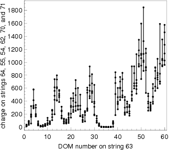
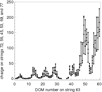
| Charges on the six nearest strings (left) and six next-to-nearest strings (right), observed when flashing at the same position on string 63. |
There is a substantial variation between the charges collected on the six surrounding strings. This variation can be due to variations in relative orientation of the flasher LEDs with respect to the surrounding strings; due to relative variation of light yield the between the different flasher LEDs, and due to some difference in distance to and depth of the six surrounding strings. The amount of variation due to these uncertainties can be quantified with an RMS of the deviation from the mean between the six surrounding strings:
A multi-pulse extraction was applied to the data, using waveforms recorded by both ATWD and FADC. The resulting pulses were binned in 25 ns bins, from 0 to 5000 ns from the flasher pulse (extracted from ATWD channel 3 of the flasher DOM). Due to high number of saturated DOMs (with a variety of problems due to high received charge) and to minimize the effect of a particular selected angular sensitivity model (of a DOM) the photon data collected on string 63 was not used in the fit.
In the above chi2 plot the value jumps each time the number of simulated flasher events is increased, and then goes down as the minimizer goes through the iterations. For the iteration steps 1-20: 1 flasher event is simulated; for 21-30: 4; for 31-40: 10. Compare with 250 flasher events in data. It is possible that the minimizer would continue to converge; the process however took 1 day and was eventually stopped. The revised value of uncertainty on py is now 20% (range 2.1 ... 3.1), as is obvious from the above plot.
| py | 1.3 | 1.4 | 1.5 | 1.6 | 1.7 | 1.8 | 1.9 | 2.0 | 2.1 | 2.2 | 2.3 | 2.4 | 2.5 | 2.6 | 2.7 | 2.8 | 2.9 | 3.0 | 3.1 | 3.2 | 3.3 | 3.4 | 3.5 | 3.6 | 3.7 | 3.8 | 3.9 | 4.0 | 4.1 | 4.2 |
| flasher | x | x | x | x | x | x | x | x | x | x | x | x | x | x | x | x | x | x | x | x | x | x | x | x | x | x | x | x | x | x |
| BG muons | x | x | x | x | x | x | x | x | x | x | x | x | x | x | x | x | x | x | x | x | x | x | x | x | x | x | x | x | x | x |
| Collection of plots for py values used in the above plot. | ||||||||||||||||||||||||||||||
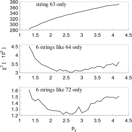 |
| chi2 for the same range of values of py as above, calculated separately for 3 groups of strings: string 63, or strings 64+55+54+62+70+71, or strings 72+56+45+53+69+77. |
The flasher fit performed for this iteration of the model was seeded with the bulk ice, while the SPICE(1) table was finalized from the minimization seeded with the AHA ice model. The following figures demonstrate that the converged solution is independent of the initial seed in most of the fitted range:
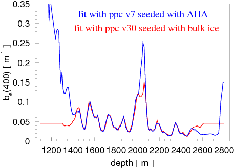
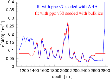
As expected, in the regions outside the detector the solutions diverge very fast as one moves farther away. Also, precision is poor in the middle of the largest dust peak. This is due to the small number of recorded pulses in data for DOMs lying within the dust peak, lack of simulation (too few flasher events were simulated for most of the iteration steps), and because the minimizer was stopped before the convergence was established (due to time constraints).
It is remarkable that both sides of the dust peak appear to have converged to a stable solution, which also correlates extremely well with the dust logger data. This is expected since the method selects all pairs of emitters and receivers that collected data, even if they are located at different depths.
Ryan sent me the following data: age vs. depth (at hole 10); dust vs. depth averaged over 6 dust logs (in holes 50, 66, 21, 52, 10, and 2), all scaled to location of hole 10; dust depth profile of logger in hole 66, which had reached the lowest depth surveyed by the dust loggers; and the table of the dust layer elevation at 19 points across the detector (in 50 meter steps).
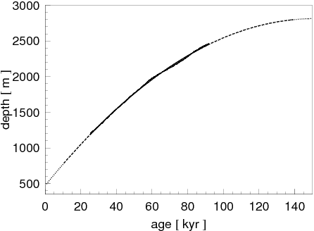
Additionally, the EDML ice core data was used to extrapolate the dust record to below the lowest dust-logger-acquired point. A simple parabola was fitted to the depth (in hole 10) vs. age data, which was used for only extrapolation beyond the tabulated range. Within the range the formula yielded the maximum error in depth (for a given age) of +- 20 m, and in age (for a given depth) of +- 1.5 kyr. The parabola extrapolation was shifted up/down to stitch smoothly to the tabulated range.
The table of dust layer elevation provided the layer shift (relief) from its position at the location of hole 50 at distance r from hole 50 along the gradient direction (225 degrees SW). I.e., the z-coordinate of a given layer at distance r is given by zr=z0+relief(z0, r). Between the grid points zr was calculated by linear interpolation in z0 and r. The equation above was solved by simple iteration resulting in a table of z0(zr)-zr, which was re-tabulated at the 6 location points of the actual dust logger records. Combined with the dust depth record at the location of hole 50 (r=0) this yields a complete description of the dust profile in and around the detector (assuming, of course, that the density of dust is the same in the same layers).
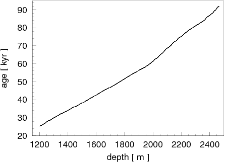
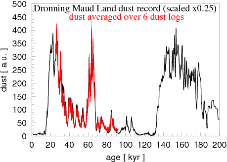
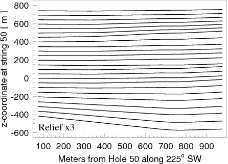
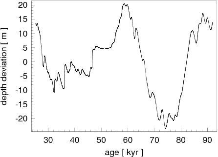
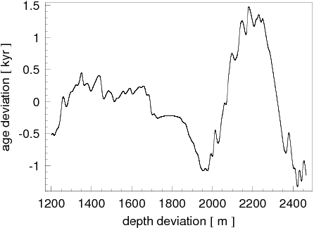
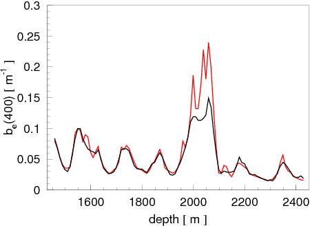
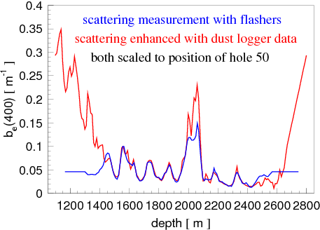
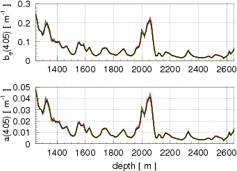
The correlation between the ice effective scattering coefficient measured with the IceCube flasher data and the average dust logger data (scaled to the location of hole 63) is phenomenal:
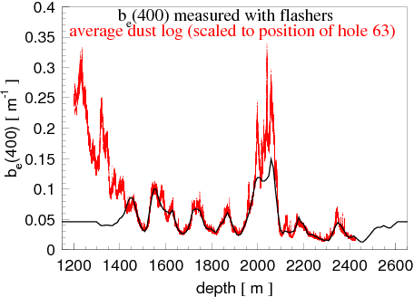
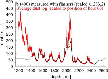
All major features match, have the right rise and falloff behavior, and are of the same magnitude. Some minor features are washed out in the flasher measurement, which was expected because of regularization terms. The dust peak is somewhat lower than in the dust logger data, which appears to be due to the minimizer having not completely converged (see the first plot on this page: the solution lines for each new iteration are progressively higher in the middle of the dust peak).
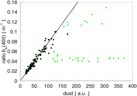
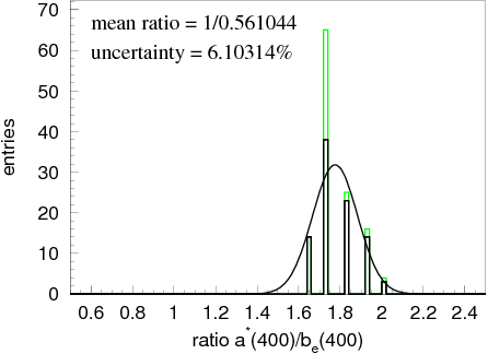
The next two plots show how the region for studying the correlation between the two sets was selected. Points outside the detector volume or those with very high scattering coefficient (shown in green) were excluded.
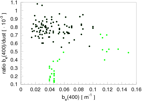
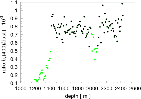
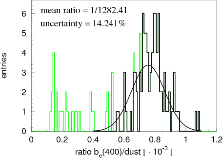
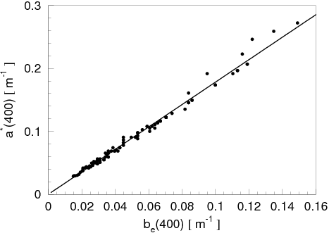
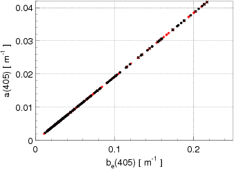
The correlation coefficient was determined and the correlation between the dust logger data and the effective scattering coefficient is shown below. The correlation is very strong in a wide range of values of the scattering coefficient, including the clearest parts of the ice. No indication of an "instrumental floor" of the dust logger (previously hinted as a possibility elsewhere) was observed. Additionally, shown below is the very strong linear correlation between the scattering and absorption coefficients (as measured in the flasher data, shown at the location of hole 63).
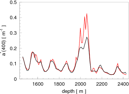
The dust logger data collected in hole 66 (the deepest log) and the ice code data from EDML were used to extend the parametrization of ice properties into the regions not covered by the average dust log:
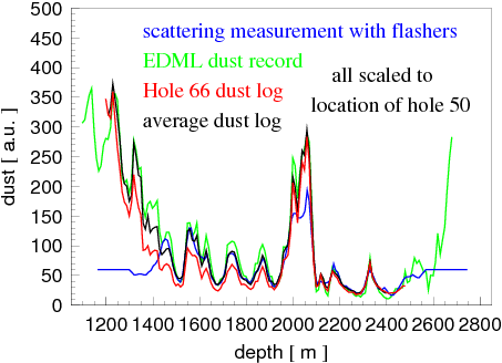
The next two plots demonstrate the overlap of such a "stitched" dust log with the effective scattering coefficient measured with the IceCube flasher data. Additionally, shown is the somewhat poorer overlap with the AHA ice model.
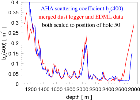
Finally, the ice table was refined with 10 more iterations of the fits to flashers (with 10 flasher events simulated):
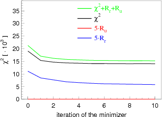
The final value of chi2 of 14045.0 is achieved (compare to 14817.7 achieved after step 39 in the chi2 plot at the top of this page).
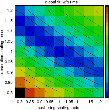
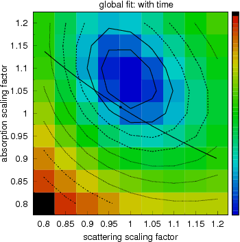
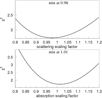
The table refined as discussed at the end of the previous section was scaled in scattering and absorption in the vicinity of the found solution to produce the likelihood profiles shown above. The fits not using the timing information have little or no ability to resolve the value of the correlation coefficient between scattering and absorption. The minimum has an extremely oblong shape, and the direction of its longest extension is determined. The point along the line drawn in this direction is chosen to minimize the likelihood that does use the timing information (which appears to have an adequate ability to resolve the correlation coefficient).
Thus, the bulk of the fits is still performed with only the total charge information, however the relationship between the scattering and absorption coefficients is now determined by fits that do use the timing information. The best point shown on the plots above determines the scaling coefficients that are applied to the ice table before the refining procedure:
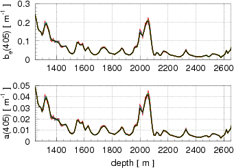
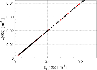

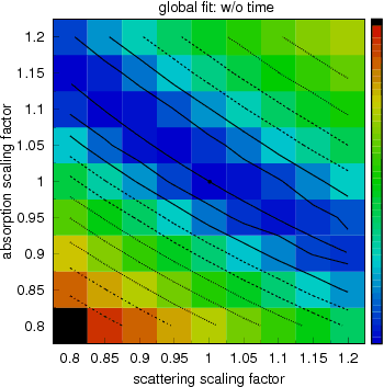
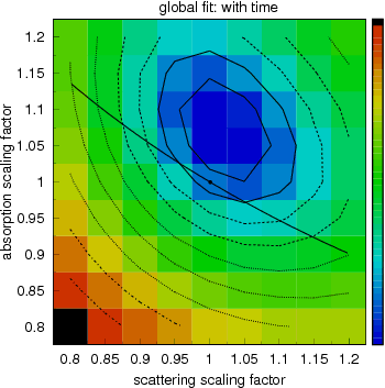
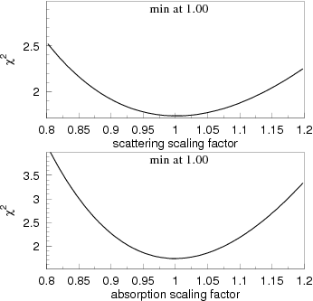
As expected, the new location of the best point is now virtually indistinguishable from (1.0, 1.0).
The method described here relies on the total charges collected by each DOM to determine the variations of the ice parameters with depth. Charge recorded by a DOM has been shown to be linear in a wide range of values (up to ~1000 p.e.) with respect to the input charge, saturation effects at the higher end being more than well covered by the systematic error belt of 20% (as used in the method described here). The more fragile (due to various observed problems) timing information is only used in a global fit to determine the correlation coefficient between scattering and absorption.
The fits could not be improved much further by allowing the scattering and absorption coefficients to vary freely (for either likelihood description: with timing or charge-only), which implies the hypothesis that the two coefficients are correlated is not only physically motivated (since both scale with concentration of dust particles in ice) but also well supported by the data.
The distance between the minimum of the likelihood using timing fits and the best value along the minimum of the likelihood that only uses charge information can be used to judge the unresolved residual uncertainty in the description of the flasher data. This uncertainty (7%, mostly in absorption coefficient, as seen from the plot above) is likely due to the approximation steps taken in describing the IceCube flashers and due to lack of some information. Here is a tentative list of such potential issues:
| Efficiency: x 1.0 no rate adjustment | hole ice | data: black ppc: blue |
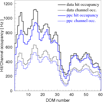 | 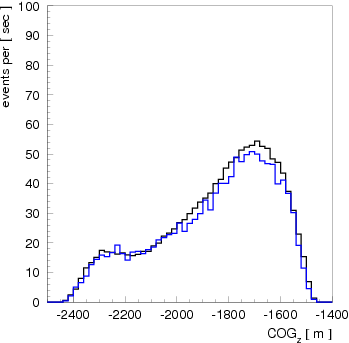 | 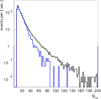 |
| Efficiency: x 0.9 no rate adjustment | hole ice | data: black ppc: blue |
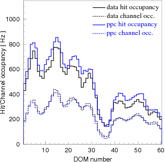 | 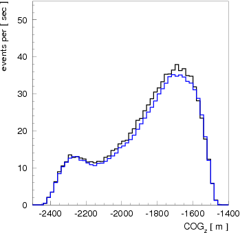 |  |
Get the new ice tables here: New! (as of 04/28/10).
  improved merging of the FADC and ATWD charges
  implemented saturation correction
  fixed the alternating ATWD bug
07/23/10 SPICELea:
??/??/10 SPICE3 (next iteration, in planning):
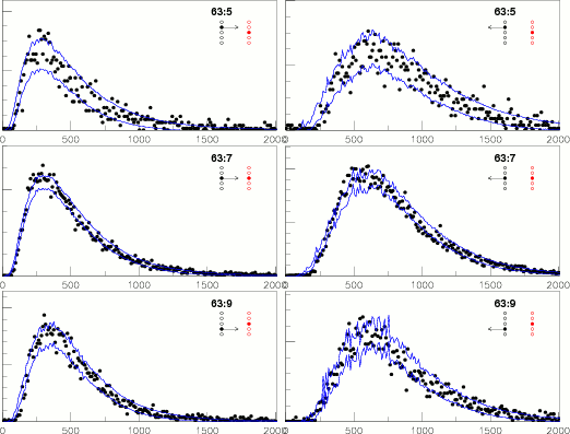
This plot shows the timing distributions received by DOM 70:7, when several DOMs/flashers on string 63 were emitting light. The blue lines indicate the simulation distorted so as to encompass most of the data points (deviating from the best fit farther than allowed by reconstructed uncertainties). It is evident already from this plot that the data is not covered by the possible simulation scenarios allowed by the fit uncertainties (two 63:7 cases disagree at the worst in the shown example). The disagreement will probably become more prominent if the statistics of the data increases.
All of emitter-receiver pairs are individually fitted (with a wrong assumption of bulk ice in between) for the best values of scattering and absorption. These values represent the best fit, so the agreement between data and simulation will get worse after data manipulation, i.e., after the individual pairs of ice parameters are replaced with the average values as shown in the plots below:
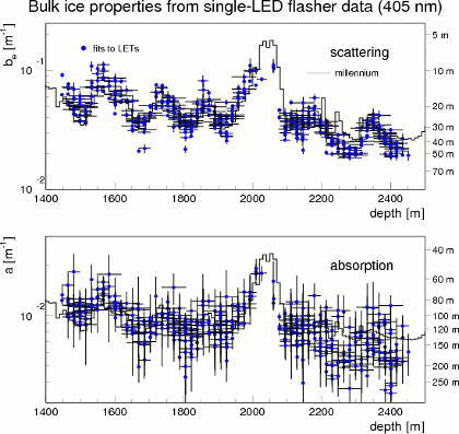
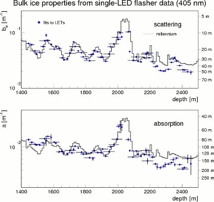
The points at any given depth disagree with each other (especially for scattering), lying far outside their respective error bars from each other. This implies that once their values are replaced with the average values for their depth, most of the time distributions will show significant disagreement between data and simulation.
The data used in AHA from the ice paper suffers from the same problem. Shown below is figure 10 from the paper; top shows all values fitted to individual emitter-receiver pairs, statistical errors not shown "for clarity"; bottom shows the averages:
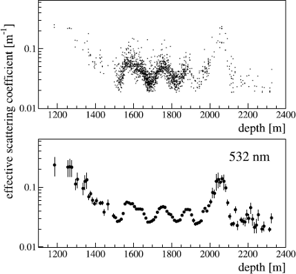
The "deconvolving" procedure that follows reportedly restores the true ice properties by enhancing the heterogeneous nature of the ice layers. However, this procedure knows nothing of the disagreement between the points lying at the same depth in the above plots. It was not designed to fit the data describing all emitter-receiver pairs, only the average scattering and absorption in each 10 meter layer. The hope of understanding the data in a statistically consistent manner is lost when the averaging is performed, i.e., before the deconvolving procedure step.
To summarize, the weakness of the method used by AHA is that the scattering and absorption parameters given at each depth are not constructed to yield the best possible representation of all data (as is done with the direct fit method of SPICE), but rather as averages of values obtained from fits to individual emitter-receiver pairs. This is especially important as these individual values are not statistically consistent with each other when compared at the same depth.
To be fair, it may be that the AHA model was constructed in such a (poor) way because the direct fit method is vastly more computationally intensive. It was only possible to implement the direct fit method recently after a substantial (100-fold) leap in performance was offered by the introduction of the GPUs. This method is now at the core of the SPICE model.