In a previous effort (SPICE) IceCube flasher data taken for all 60 DOMs of string 63 was used to obtain the ice properties at the detector depths (scattering and absorption at 405 nm average flasher wavelength). This page describes a near-perfect correlation of that measurement with the dust logger data collected in 6 of the IceCube holes by Ryan Bay. It was possible to use this correlation to extend the flasher measurement to depths above and below the detector, and to horizontal locations in the detector other than those near string 63, taking into account the detailed layering structure measured with the dust loggers. A new ice model (SPICE2) that takes into account both the flasher and dust logger measurements is introduced and the fitted tables are provided. A preliminary study of the background muons performed by a stand-alone (not icetray) simulation demonstrates a near-perfect description in historically troublesome variables (OM occupancy, COGz, and Nch). Detailed studies within icetray are underway and will be discussed elsewhere.
South Pole ICE (SPICE) model is based on IceCube data collected when flashing DOMs on string 63. For the summary of this measurement go here. The ice table linked from the page is based on the likelihood minimization fits seeded with the AHA model. Thus, this model relies on AHA to extrapolate the absorption and scattering coefficients to the region outside the detector volume.
This page introduces the second iteration of SPICE, or SPICE2 model (read spicetwo) that relies on the dust logger and ice core data to extrapolate the ice propertied to the region outside the detector volume. It is envisioned that there will be one more iteration, SPICE3 (read spicecube) that will improve the agreement with the standard candle data. It is hypothesized that this may require a new set of parameters of the wavelength dependence of the scattering and absorption coefficients.
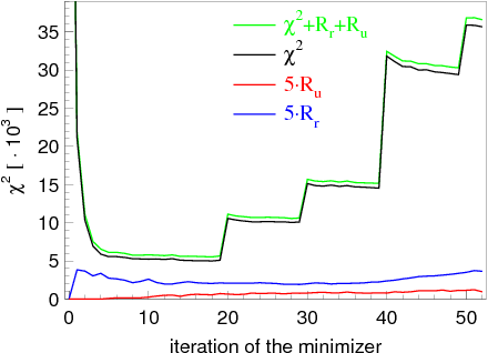
The model is based on the same minimization procedure as used for the first iteration of SPICE, but seeded with the bulk ice properties and performed with the ppc software release version v17 (vs. previously used v7) that had fixed the hdh bug (which turned out to be a very minor issue). The new version is several times faster than the old one, which allowed for more iterations to be performed with more precision:


In the above chi2 plot the value jumps each time the number of simulated flasher events is increased, and then goes down as the minimizer goes through the iterations. For the iteration steps 1-20: 1 flasher event is simulated; for 21-30: 4; for 31-40: 10; for 41-50: 100; and for the iteration steps 51 and 52: 250 flasher events were simulated (same as in data). It is possible that the minimizer would continue to converge; the process however took 2 weeks and was eventually stopped. The revised value of uncertainty on py is now 15%, as is obvious from the above plot.
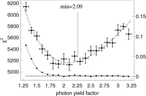
The 10% cable shadowing was taken into account during the simulation, reducing the OM efficiently from 100% to 90%. This is reflected in the photon yield factor at the minimum that is 10% higher than the previously reported value. This behavior is expected as the DOM efficiency comes into the calculation only in a combination with the total number of emitted photons, thus making it impossible to decouple the two.
| py | 1.3 | 1.4 | 1.5 | 1.6 | 1.7 | 1.8 | 1.9 | 2.0 | 2.1 | 2.2 | 2.3 | 2.4 | 2.5 | 2.6 | 2.7 | 2.8 | 2.9 | 3.0 | 3.1 | 3.2 |
| flasher | x | x | x | x | x | x | x | x | x | x | x | x | x | x | x | x | x | x | x | x |
| BG muons | x | x | x | x | x | x | x | x | x | x | x | x | x | x | x | x | x | x | x | x |
| Collection of plots for py values used in the above plot. | ||||||||||||||||||||
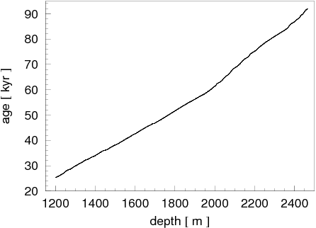
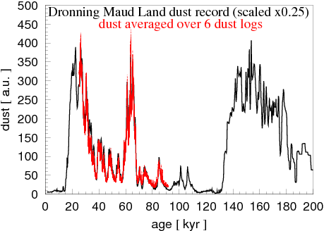
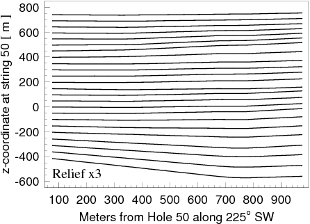
Ryan sent me the following data: age vs. depth (at hole 10); dust vs. depth averaged over 6 dust logs (in holes 50, 66, 21, 52, 10, and 2), all scaled to location of hole 10; dust depth profile of logger in hole 66, which had reached the lowest depth surveyed by the dust loggers; and the table of the dust layer elevation at 19 points across the detector (in 50 meter steps).
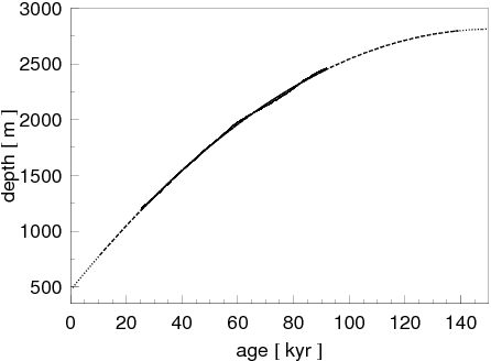
Additionally, the EDML ice core data was used to extrapolate the dust record to below the lowest dust-logger-acquired point. A simple parabola was fitted to the depth (in hole 10) vs. age data, which was used for only extrapolation beyond the tabulated range. Within the range the formula yielded the maximum error in depth (for a given age) of +- 20 m, and in age (for a given depth) of +- 1.5 kyr. The parabola extrapolation was shifted up/down to stitch smoothly to the tabulated range.
The table of dust layer elevation provided the layer shift (relief) from its position at the location of hole 50 at distance r from hole 50 along the gradient direction (225 degrees SW). I.e., the z-coordinate of a given layer at distance r is given by zr=z0+relief(z0, r). Between the grid points zr was calculated by linear interpolation in z0 and r. The equation above was solved by simple iteration resulting in a table of z0(zr)-zr, which was re-tabulated at the 6 location points of the actual dust logger records. Combined with the dust depth record at the location of hole 50 (r=0) this yields a complete description of the dust profile in and around the detector (assuming, of course, that the density of dust is the same in the same layers).
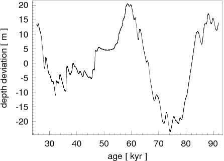
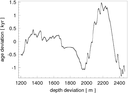
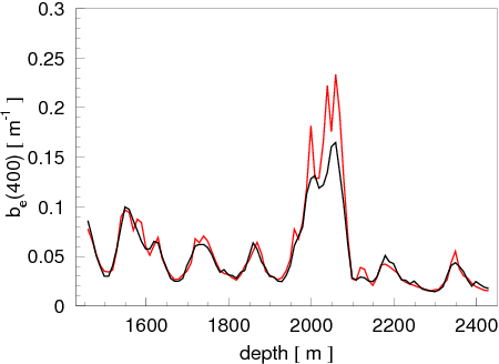
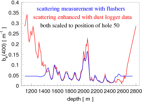
The correlation between the ice effective scattering coefficient measured with the IceCube flasher data and the average dust logger data (scaled to the location of hole 63) is phenomenal:
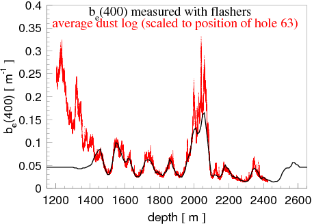
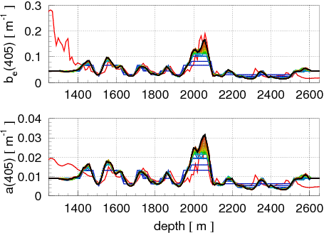
All major features match, have the right rise and falloff behavior, and are of the same magnitude. Some minor features are washed out in the flasher measurement, which was expected because of regularization terms. The dust peak is somewhat lower than in the dust logger data, which appears to be due to the minimizer having not completely converged (see the first plot on this page: the solution lines for each new iteration are progressively higher in the middle of the dust peak).
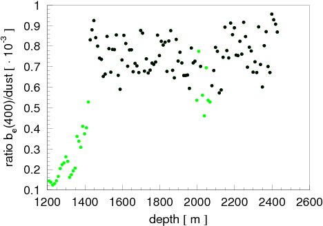
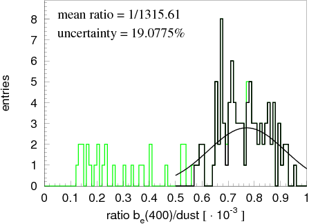
The next two plots show how the region for studying the correlation between the two sets was selected. Points outside the detector volume or those with very high scattering coefficient (shown in green) were excluded.
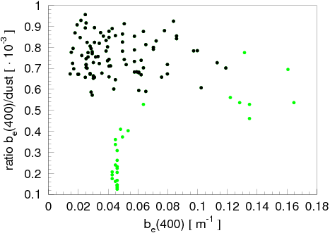
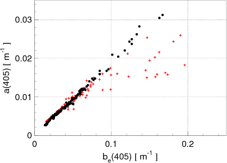
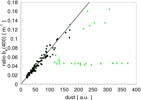
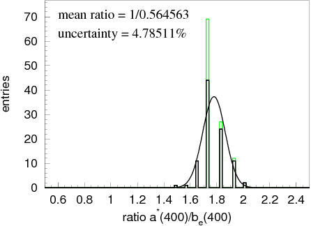
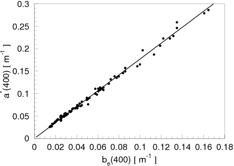
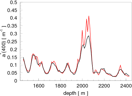
The correlation coefficient was determined and the correlation between the dust logger data and the effective scattering coefficient is shown below. The correlation is very strong in a wide range of values of the scattering coefficient, including the clearest parts of the ice. No indication of an "instrumental floor" of the dust logger (previously hinted as a possibility elsewhere) was observed. Additionally, shown below is the very strong linear correlation between the scattering and absorption coefficients (as measured in the flasher data, shown at the location of hole 63).
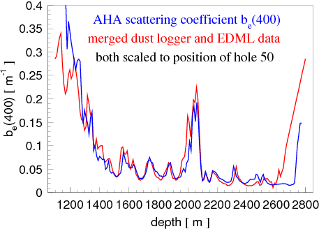
The dust logger data collected in hole 66 (the deepest log) and the ice code data from EDML were used to extend the parametrization of ice properties into the regions not covered by the average dust log:
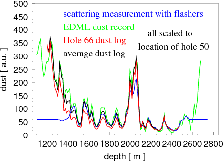
The next two plots demonstrate the overlap of such a "stitched" dust log with the effective scattering coefficient measured with the IceCube flasher data. Additionally, shown is the somewhat poorer overlap with the AHA ice model.
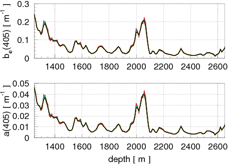
Finally, the ice table was refined with 10 more iterations of the fits to flashers (with 10 flasher events simulated):
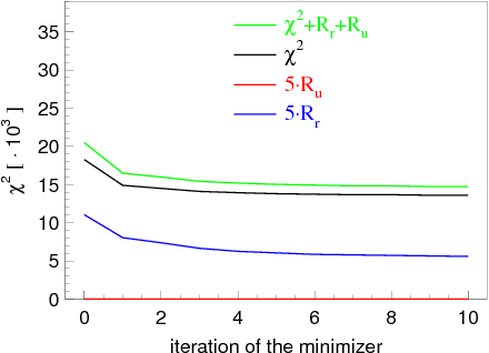
The final value of chi2 of 13616.7 is achieved (compare to 14526.8 achieved after step 39 in the chi2 plot at the top of this page).
The flasher fit performed for this iteration of the model was seeded with the bulk ice, while previous table was finalized from the minimization seeded with the AHA ice model. The following figures demonstrate that the converged solution is independent of the initial seed in most of the fitted range:
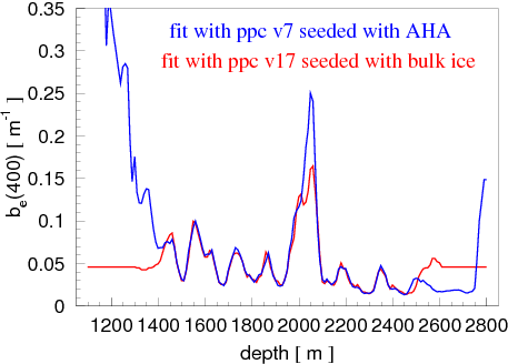
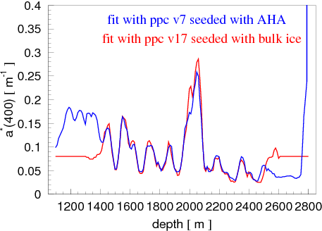
As expected, in the regions outside the detector the solutions diverge very fast as one moves farther away. Also, precision is poor in the middle of the largest dust peak. This is due to the small number of recorded pulses in data for DOMs lying within the dust peak, lack of simulation (too few flasher events were simulated for most of the iteration steps), and because the minimizer was stopped before the convergence was established (due to time constraints).
It is remarkable that both sides of the dust peak appear to have converged to a stable solution, which also correlates extremely well with the dust logger data. This is expected since the method selects all pairs of emitters and receivers that collected data, even if they are located at different depths.
The effect of the hdh bug appears to be insignificant. It was expected that the cumulative calculated photon length might be affected if the photon crossed more than 2 ice layers between the consecutive scattering points.
The effect of more iterations with higher number of simulated flasher events is evident in the figures above: the peak-to-valley amplitude is larger in the new model. This is to be expected, as the role of the regularization terms was diminished somewhat as the precision of the main likelihood term (describing the difference between data and simulation) rose (with 10x more simulated events).